Download

1 / 14
150 likes | 368 Vues
Project: Numerical Solutions to Ordinary Differential Equations in Hardware. Joseph Schneider EE 800 March 30, 2010. Ordinary Differential Equations. Function with one independent variable and derivatives of the dependent variable Eg . y’ = 1 + y/x

E N D
Project: Numerical Solutions to Ordinary Differential Equations in Hardware Joseph Schneider EE 800 March 30, 2010
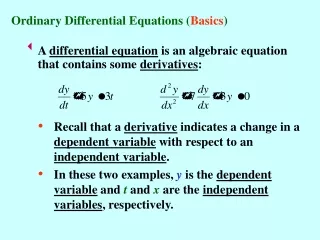
Ordinary Differential Equations • Function with one independent variable and derivatives of the dependent variable • Eg. y’ = 1 + y/x • Requires some initial condition in order to be solved • Eg. y(1) = 2
Ordinary Differential Equations • Found in many areas of engineering • Radioactive decay, heat equation, motion… • In electrical engineering, charge, flux, voltage, current, all intertwined by differential equations
Ordinary Differential Equations • In some cases, original equation can be derived with relative ease; Exact solutions are then available • In other cases, we will only have the ODE to work with • Numerical solutions have been developed to deal with these cases
Ordinary Differential Equations • Most basic case: Euler’s Method • Selecting a step size h, iterate from initial value to desired value using the derivative function
Ordinary Differential Equation • Euler’s Method most basic case – Simple, but inaccurate • Variety of other methods that have been developed
Ordinary Differential Equations • Error directly linked with step size • As step size decreases, error decreases; However, takes longer for process to complete • Implemented in software (eg. Matlab), more accurate methods take several seconds to complete for smaller scale cases; Several minutes for larger cases
Ordinary Differential Equations • Original project goal: Implement the Runge-Kutta 4th order method in hardware for improved speed
Project • Euler’s method also implemented for comparisons on area, timing, and accuracy. • Current implementation: Uses fixed-point number representation, state machine • Further steps on this implementation • Variable-point number representation to improve accuracy • Modify for parallelism to examine impacts on area, timing
Project • Second implementation: Error-controlled design of Runge-Kutta method • Error is specified at beginning of process, step size is varied to ensure final result meets error specifications
Project • For second implementation, desired to use a hardware design to improve on bottleneck of software design • Comparisons to software on time vs. error threshold