Download
1 / 50
500 likes | 709 Vues
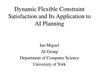
Dynamic Flexible Constraint Satisfaction and Its Application to AI Planning. Ian Miguel AI Group Department of Computer Science University of York. Outline. Part I Constraint Satisfaction. Weaknesses/Remedies. Dynamic Flexible Constraint Satisfaction. Part II AI Planning.

E N D
Dynamic Flexible Constraint Satisfaction and Its Application toAI Planning Ian Miguel AI Group Department of Computer Science University of York
Outline • Part I • Constraint Satisfaction. • Weaknesses/Remedies. • Dynamic Flexible Constraint Satisfaction. • Part II • AI Planning. • Flexible Planning. • Plan Synthesis via dynamic flexible CSP.
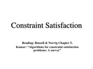
Constraints • A natural means of knowledge representation. • x + y = 30 • Adjacent countries on the map cannot be coloured the same. • The helicopter can carry one passenger. • The maths class must be scheduled between 9 and 11 am.
Specify allowed combinations of assignmentsof values to variables. The Constraint Satisfaction Problem (CSP) • Given: • A set of variables. • Each variable has an associated finite domain of potential values. • A set of constraints over these variables. • Find: • A complete assignment of values to variables that satisfies all constraints.
Applications • Combinatorial Mathematics. • Fault diagnosis. • Machine vision. • Planning. • Scheduling. • Systems Simulation. • Csplib.org
These unary constraints determine the domains in this simple example. Example CSP – Course Scheduling • Decide the number of lecture, exercise and training sessions. • So we need 3 variables. • Constraints: • There must be a total of 8 sessions. • Professor A will give 4 or 5 lectures. • Dr B will give 3 or 4 exercise sessions. • There must be 1 or 2 training sessions.
Solving CSPs • Most often depth-first search (I.e. Backtrack). • Select an unassigned variable. • Select a value compatible with all previously assigned variables. • If no such value, backtrack and find a new value for previous variable… Root 1st variable 2nd variable
Constraints: • There must be a total of 8 sessions. • Professor A will give 4 or 5 lectures. • Dr B will give 3 or 4 exercise sessions. • There must be 1 or 2 training sessions. Course Scheduling: A Solution • Lectures = 4 • Exercise = 3 • Training = 1
The Problem Changes… • Constraints: • There must be a total of 8 sessions. • Professor A will now give 3 or 4 lectures. • Dr B agrees to give 4 or 5 exercise sessions. • There must be 1 or 2 training sessions. • The solution to the old problem: • Lectures = 4 • Exercise = 3 • Training = 1
Weakness 1: Static Formulation • Classical CSP has no way of dealing with this change gracefully. • Naively we can solve the new problem from scratch. • This wastes all work on the old problem! • So? • We use an extension called dynamic CSP.
Dynamic CSP • A dynamic environment is viewed as a sequence of static CSPs. • Linked by: • Restriction (constraints added) • Relaxation (constraints removed)
Solving Dynamic CSPs • Oracles: • Start from scratch. • Previous solution guides value assignment. • Local Repair: • Start from previous solution. • Modify individual assignments until find a solution. • Constraint Recording: • Record new constraints during search. • Carry new constraints over to future problems to restrict search there.
Incompatible withsolution to problem 1 Course Scheduling Problem 1 Problem 2 Solution: Lectures = 4 Exercise = 3 Training = 1 Solution: Lectures = 3 Exercise = 4 Training = 1 • In problem 2: • Dr B agrees to give 4 or 5 exercise sessions. • Repair method: • Start with violated exercise constraint: Exercise = 4 • Then repair violated sum constraint: Lectures = 3
The Problem Changes Again… • Constraints: • There must be a total of 7 sessions. • Professor A will give 3 or 4 lectures. • Dr B will give 4 or 5 exercise sessions. • There must be 1 or 2 training sessions. • This problem has no solution.
Weakness 2: Hard Constraints • Classical CSP has no way of finding a compromise. • Constraints are hard: • Imperative: Valid solution must satisfy all of them. • Inflexible: Constraints wholly satisfied or wholly violated. • So? • We use an extension called flexible CSP.
Flexible CSP • An umbrella term for a variety of methods. • Max-CSP: Maximise the number of satisfied constraints/Minimise violations. • Weighted Max-CSP. • Weighted Preference. • Fuzzy CSP. • General frameworks: • Partial CSP, Valued CSP, Semi-ring CSP.
Solving Flexible CSPs • Branch and bound is most common technique. • Search for a first solution (minimise violations). • Use this as a bound on future solutions. • As soon as current search branch can be shown to be equal or exceed the bound, prune it. • When a new solution is found, use as new bound, etc… Equals bound: 3 violatedalready. Prune. New boundE.g. 3 violatedconstraints.
Incompatible withsolution to problem 2 Course Scheduling Problem 2 Problem 3 Solution: Lectures = 3 Exercise = 4 Training = 1 • In problem 3: • There must be a total of 7 sessions. • Max-CSP: Pretty good solution – only 1 violated constraint. • Or attach priorities/preferences to each constraint.
The Gap in the Market • Dynamic CSP research is founded almost exclusively on hard constraints. • Flexible CSP research is founded almost exclusively on static problems. • We want to combine the two to bring to bear the benefits of both.
Solution methods Dynamic Flexible CSP • Also an umbrella term for a variety of methods. Dynamic CSP Techniques Restriction Relaxation Recurrent Activity … Max DFCSP Instance WeightedMax FlexibleCSPTechniques Weighted Preference Fuzzy …
Fuzzy rrDFCSP • Restriction/Relaxation DCSP + Fuzzy CSP. • Fuzzy CSP: • A totally ordered satisfaction scale. • Endpoints signify total violation/satisfaction. • Constraints modelled by fuzzy relations: map variable assignments to points in the scale. • Overall satisfaction determined by fuzzy conjunction: the min operator.
Two Algorithms • Dynamic version of a flexible CSP algorithm. • Using oracles method. • Flexible version of a dynamic CSP algorithm. • Flexible Local Changes. • Each algorithm has several variants, which do an increasing amount of work to spot dead ends early.
Flexible Local Changes • Complete Local repair algorithm. • Divides Variables into three sets: • Assigned & Fixed. • Assigned & Not Fixed. • Unassigned. • Uses these sets to control search procedure.
Flexible Local Changes: Operation 1 2 3 Sub-problemsolved. … • Maintain a bound on bestsolution found for eachsub-problem. 1 2 3 1 2 3 1 2 3 1 2 3 1 2 3 Sub-sub problemsolved. • Assigned & Fixed. • Assigned & Not Fixed. • Unassigned.
Experiments • We wanted to investigate: • The structure of fuzzy rrDFCSPs. • The relative performance of the algorithms. • We varied: • Problem size. • Connectivity. • Proportion of variables related by a constraint. • Constraint tightness. • Proportion of disallowed value combinations. • Satisfaction scale size. • The amount of change between instances. • Each sequence contains 10 problems.
Experiments: Measurements • Constraint checks. • Every time we query a constraint for the satisfaction degree of an assignment. • Search nodes. • Every time we assign a value to a variable. • Size of search tree. • Solution stability. • Proportion of assignments that remain the same between instances.
Results: Search Effort • Mean over 3 sequences of 10 instances. • Scale size: 3, Change 1 constraint between instances. • Instance size: 20 variables, connectivity: 0.25
Search Effort: Trends • Branch and bound finds solutions more efficiently than FLC. • BB has a more rigid search structure. • This allows stronger inferences to be made at each node in the search tree. • Result: BB spots dead ends earlier. • Algorithm variants: • Doing more work to spot dead ends guarantees a smaller or equal-sized search tree. • But often costs more in terms of constraint checks.
Search Effort: Trends • Phase transition behaviour. • Increasing some parameters generally increases difficulty: • Problem size. • Connectivity. • Size of satisfaction degree scale. • Amount of change between instances.
Results: Stability • Scale size: 3, Change 1 constraint between instances • Problem size: 20 variables, connectivity: 0.25
Stability: Trends • FLC produces more stable solutions than BB. • Both algorithms prefer stable assignments where possible. • FLC actively seeks to leave areas of the previous solution undisturbed. • Variants: More work to spot dead ends means more stability. • Extra work gives us a better idea of the utility of potential assignments. • Can reveal that they are no better than our preferred stable assignment.
Utility of Dynamic Information • We tested `crippled’ versions of the algorithms. • Branch and bound loses its oracle. • FLC starts from an empty assignment. • Crippled versions: • Explore significantly larger search trees. • Give significantly lower solution stability. • Extent varies according to the particular dynamic sequence.
Part II Application to AI Planning
AI Planning • Plan: Course of action to achieve pre-specified goals. • Components of a planning problem: • Plan objects. • Initial state. • Goal state. • Operators. c3 guard1 r2 r3 pkg1 pkg2 m1 m2 c1 c2 c4 r1
Characteristics of AI Planning • Inflexible operators. • Imperative goals. • Suffers from similar problems to classical CSP. • If no `perfect’ solution, no plan returned. • We want to give the planner the ability to compromise.
Preference Can relax, with associated damage to resultant plan Imperative Flexible Planning • Incorporate preferences into operators and goals. • Model both via fuzzy relations: • Map from preconditions onto a totally ordered satisfaction scale. • Load-truck operator has preconditions: • Truck and package in same place. • Guard must be present.
Example c3 L={l , l1, l2, lT} guard1 r2 r3 pkg1 pkg2 • Goals: • Both packages to c4. • pkg2 is worth less, don’t deliver: l1 • Guard to c3. • Can also leave guard at c2 or c4: l2 m1 m2 c1 c2 c4 r1
Example c3 L={l , l1, l2, lT} guard1 r2 r3 pkg1 pkg2 • Operators: • Drive-truck. • Avoid mountains or: l1 • Load/Unload-truck. • For valuable package, guard present or: l2 • Guard-boards/leaves-truck. m1 m2 c1 c2 c4 r1
Inconsistent: • Preconditions • Effects Graphplan • Solution procedure for classical planning problems. • Constructs/analyses a planning graph. • Forward phase extends planning graph until goals found. • Add binary mutex constraints between actions/propositions that conflict. • Backward phase extracts valid plan. Actions1 Propositions1 . . . Initial Conditions . . . . . .
The Flexible Planning Graph • Actions annotated with their satisfaction degrees. Actions1 Propositions1 . . . l2 . . . l3 . . . l1
The CSP Viewpoint • Variables: proposition nodes. • Domains: actions who assert these propositions as effects. • Constraints: Binary mutex + Unary fuzzy. Actions1 Propositions1 . . . l2 . . . l3 . . . l1
Plan Synthesis via Fuzzy rrDFCSP • Goals, and their domains form a first sub-problem. • Action pre-conditions specify new sub-problems… Goal Sub-problem • Solutions at level n are likely to intersect. • So, problems at level n-1 form a related sequence: • Each level is a DFCSP.
Guiding Overall Search • Goal: Solve as few sub-problems as possible. • Generate memosets from unsolvable sub-problems. • Propagate memosets up the level hierarchy. Goal Sub-problem
4-step Solution c3 L={l , l1, l2, lT} guard1 r2 r3 pkg1 pkg2 • Load-truckpkg1truckl2. • Drive-trucktruckc1 to c2 via r1 lT. • Drive-trucktruckc2 to c4 via m2 l1. • Unload-truckpkg1truckl2. m1 m2 c1 c2 c4 r1 Satisfaction: l1
6-step Solution c3 L={l , l1, l2, lT} guard1 r2 r3 pkg1 pkg2 • Load-truckpkg1truckl2. • Drive-trucktruckc1 to c2 via r1 lT. • Load-truckpkg2trucklT. • Drive-trucktruckc2 to c3 via r2 lT. • Drive-trucktruckc3 to c4 via r3 lT. • Unload-truckpkg1truckl2, pkg2trucklT. m1 m2 c1 c2 c4 r1 Satisfaction: l2
Compromise-free Solution c3 L={l , l1, l2, lT} guard1 r2 r3 pkg1 • 10 steps. • First collect the guard. • Return to load pkg1. • Use the main roads to deliver both packages and guard. pkg2 m1 m2 c1 c2 c4 r1
Flexible Graphplan: Observations • It is more expensive to search for a range of plans than for one compromise-free plan. • But it is often possible to find short, compromise plans quickly. • Supports anytime behaviour. • Range of plans trade length versus number and severity of the compromises made.
Conclusions • Dynamic flexible constraint satisfaction combines two extensions to classical CSP. • Multiple instances of DFCSP. • Considered fuzzy rrDFCSP in detail. • Two solution procedures (with variants). • Flexible planning. • Plan synthesis via hierarchical decomposition and fuzzy rrDFCSP.
Future Work • We have examined one instance of DFCSP in detail. • Examine other instances. • Modify existing solution techniques/consider new ones (e.g. local search). • Other applications. • Compositional Modelling [Keppens 2002]. • Dynamic Scheduling. • Interactive configuration…
Acknowledgements • Qiang Shen, University of Edinburgh. • Peter Jarvis, SRI International.