Sparse LCS Common Substring Alignment

1. Sparse LCS Common Substring Alignment Gad M .Landau, Baruch Schieber and Michal Ziv-Ukelson CPM03 張耿豪 王姵瑾 吳亭範

2. Outline • Introduction • Preliminaries • The algorithm • Totally Monotone Rectangular Matrix • Conclusions and Open Problems

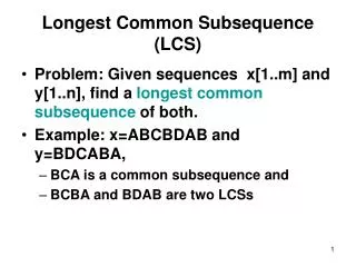
3. Input: a set of strings S1, S2, …, Scand a target string T Output: the similarity of all strings Si with T Under LCS similarity metric Ex: S1=ababaa S2=aabbb T=abab Sim(S1, T) = 4 Sim(S2, T) = 3 Common Substring Alignment

4. Application • Molecular biology… • Search the most similar strings in database

5. Main idea • Y is the common substring of Si • Don’t compute of the similarity between Y and T over and over again. • The sparsity of LCS

6. B C B A D B D B B B O5 3 O4 2 O8 4 I0 0 I1 1 I2 1 I3 1 I5 1 I4 1 I7 1 I6 1 I8 1 O7 4 O6 4 O0 0 O1 1 O2 1 O3 2 D B B T DP Graph Varies by Si Bi G Y Si Speed up Fi Same structure

7. Three stages • In Common Substring Alignment • Preprocessing stage • Encoding stage • Alignment stage

8. Preprocessing stage • Parsed for the optimal common substring… compromise • Si = Bi Y Fi T = “BCBADBDCD” Y= “BCBD” S1= “BC BCBD C” B1= “BC” F1 = “C” S2= “E BCBD DBCBD A” B2a = “E” F2a= “DBCBDA” B2b = “EBCBDD” F2b=“A”

9. In this paper • We assume that Y is given. We focus on the following two stages.

10. A data structure is constructed which encodes the comparison of Y with T Goal: to speed up alignment stage T B C B A D B D B Bi B I0 0 I1 1 I2 1 I3 1 I4 1 I5 1 I6 1 I7 1 I8 1 G B Y D B O0 0 O1 1 O2 1 O3 2 O8 4 O4 2 O5 3 O6 4 O7 4 Fi B Encoding Stage

11. Align between Si and T Use the pre-compiled data-structure to align Y and T T B C B A D B D B Bi B I0 0 I1 1 I2 1 I3 1 I4 1 I5 1 I6 1 I7 1 I8 1 G B Y D B O0 0 O1 1 O2 1 O3 2 O8 4 O4 2 O5 3 O6 4 O7 4 Fi B Alignment Stage

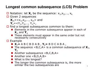
12. Notation • n = |Si| = |T| • L = max{LCS[T, Si]} • Ly=|LCS[T, Y]| • (Ly ≤ |Y|, Ly ≤ L, L ≤ n)

13. Previous result Encoding stage O(n2+n|Y|) Alignment stage O(n) (SIAM 2001) In this paper Encoding stage O(nLy) Alignment stage O(L) Results Sparcity of LCS: Ly << |Y|, L << n

14. I0 0 I1 1 I2 1 I3 1 I4 1 I5 1 I6 1 I7 1 I8 1 T B Y D G B O0 O1 O2 O3 O8 O4 O5 O6 O7 Our goal now ?

15. Auz= substring of A from index u to z, 1≤u≤z≤n I[j]=|LCS[T1j, Bi]| (0,0) 到input row I 的第j個vertex的optimal path‘s weight O[j]=|LCS[T1j, BiY]| B C B A D B D B Bi B I0 0 I1 1 I2 1 I3 1 I4 1 I5 1 I6 1 I7 1 I8 1 B Y D B O0 0 O1 1 O2 1 O3 2 O8 4 O4 2 O5 3 O6 4 O7 4 Fi B DP Graph G

16. In a given row in the DP graph,LCS has two properties 遞增 每一步頂多增加1 增加一個match B D B A D B D C B C B 2 2 2 1 1 1 1 1 0 Observation

17. I[j]=|LCS[T1j, Bi]| (0,0) 到input row I 的第j個vertex的optimal path‘s weight O[j]=|LCS[T1j, BiY]| For k = 0,…,L PI[k] Row I 中, weight k 的block的起始index 由DP graph中(0,0)到 row I,weight為k且最左邊的path PO[k] Row O 中, weight k 的block的起始index 由DP graph中(0,0)到 row O,weight為k且最左邊的path Some alternative…

18. PI[k] and PO[k] are sufficient to represent I[j] and O[j] T I0 0 I1 1 I2 1 I3 1 I4 1 I5 1 I6 1 I7 1 I8 1 G B Y D B O0 0 O1 1 O2 1 O3 2 O8 4 O4 2 O5 3 O6 4 O7 4 Therefore… PI = 0 1 PO = 0 1 3 5 6

19. Claim • Only the positions PI[r] are sufficient for computing PO[k], r, k = 0,…,L Row I中, 不是PI[r]的index在Row O所能達到的結果,PI[r’]也能達到,甚至更好 • Proof • i1 = PI[k], i3=PI[k+1] if defined • For any index i2, i1<i2<i3 (I[i1]=I[i2]), 對Row O的index j I[i1]+|LCS[Ti1+1j,Y]| ≥ I[i2]+|LCS[Ti2+1j,Y]| (通過i1所走的path至少比通過i2所走的path好)

20. Given vector PI, compute vector PO! B Y D B Objective now!! T PI = 0 1 ? PO

21. Observation • When compute PO[k], only PI[r] are candidates, 0≤r≤k • 只有通過row I weight≤k的 path才有可能造成row O的k-path

22. PO

23. The Algorithm Encoding Stage Alignment Stage 消消樂 另一半 最近邊界 Total Monotone in O(n) S in O(n|LCS(Y,T)|) Construct LEFT in O(n) Column Minima of LEFT in O(n)

24. PI 0 1 2 Bi Y Fi PO 0 1 2 3 4 B C B A D B D C 0 B A B D B

25. T PI[r] j Bi r PI[r] PI k-r = LCS[TjPI[r]+1,Y] Y PO PO[k] Fi

26. r r+1 r-1 PI[r] PI[r+1] PI[r-1] k-r-1 k-r k-r+1 PO[k]=? PO[k]=? PO[k]=? T Find Optimal SubPath Bi PI Y PO Fi

27. r r+1 r-1 PI[r] PI[r+1] PI[r-1] k-r-1 k-r k-r+1 PO[k]=? PO[k]=? PO[k]=? Encoding Stage • Preprocessing: Si unknown • Table S: alignment of T, Y Bi PI Y PO Fi S[i, w] = min{j | |LCS[Tji+1, Y]| = w}

28. Algorithm S[i, w] = min{j | |LCS[Tji+1, Y]| = w} for i = 0 to |T| S[i, 0] i for k = 0 to … S[i, k+1] = S[i, k] + d next k next i

29. 起點 weight Observation S[1,0] = 1 S[1,1] = S[1,0] + 最近邊界距離* = 1 + 1 S[1,2] = S[1,1] + 最近邊界距離* = 2 +2 =4 • S[i, k+1] = S[i, k] + d T C B A D B D C B B A Y B D B 1 2 3 4 5 6 7 8 9

30. 尋找最近邊界 • O( |Alphabet| * (|Y|+|T|) ) preprocessing • O(1) finding next

31. Preprocessing • Finding all matches • foreach alphabet, scan Y, T for position • matches  現(B in Y) cross 現(B in T) • construct a fastfind structure T C B A D B D C B B A Y B D B

32. Algorithm S[i, w] = min{j | |LCS[Tji+1, Y]| = w} for i = 0 to |T| S[i, 0] i for k = 0 to O(|LCS(Y,T)|) S[i, k+1] = S[i, k] + d next k next i

33. i The Inner Loop—O(|LCS(Y,T)|) T B C B A D B D C B A Y B D B S[i, k+1] = S[i, k] + d

34. Complexity • Assume |T| > |Y| • preprocessing O( |Alphabet| * (|Y|+|T|) ) • The inner loopO( |LCS(Y,T)| ) • The outter loopO(|T|) • OverallO( |T|*|LCS(Y,T)| ) for i = 0 to |T| S[i, 0] i for k = 0 to O(|LCS(Y,T)|) S[i, k+1] = S[i, k] + d next k next i

35. The Algorithm Encoding Stage Alignment Stage 消消樂 另一半 最近邊界 S in O(n|LCS(Y,T)|) Construct LEFT in O(n) Column Minima of LEFT in O(n)

36. r r+1 r-1 PI[r] PI[r+1] PI[r-1] k-r-1 k-r k-r+1 PO[k]=? PO[k]=? PO[k]=? Alignment Stage PO[k] = minkr=0{ S[ PI[r], k-r] } T Bi PI Y PO Fi

37. Construction of Left(1) PO[k] = minkr=0{ S[ PI[r], k-r] }

38. Construction of Left(2) PO[k] = min{ }

39. Construction of Left(3) PO[L]=min{} PO[0]=min{} PO[1]=min{}

40. Undefined Region in LEFT[][] PI[r+1] PI[r-1] PI[r] PI k-r-1 k-r k-r+1 PO PO[k]=? PO[k]=? PO[k]=? S[i, w] = min{j | |LCS[Tji+1, Y]| = w} 起點 增加的weight PO[L]=min{} PO[0]=min{} PO[1]=min{}

41. Good Property of Left[][] • Totally Monotone Rectangular Matrix Convex Concave Or

42. Reduced Problem • The minimum value of each column • nxn total monotone matrix  O(n)

43. Find Column Minima Recursively Minima(Am×n) Bn×n消(Am×n) If #row(Bn×n) = 1 return the positions of minima 另一半by Minima(半(B)) return the positions of minima

44. 半 消 半 消 半 消

45. The Algorithm Encoding Stage Alignment Stage 消消樂 另一半 最近邊界 S in O(n|LCS(Y,T)|) Construct LEFT in O(n) Column Minima of LEFT in O(n)

46. ≤ 消::m×n  n×n n Type A: 自亂陣腳 Type B: 全排覆沒 ≤ ≤ m >

47. 消 at the n-th row n Type C: 敵前投降 m ≤

48. Complexity of 消—O(m) • At most m-n deletions • B全排覆沒+C敵前投降 = O(m-n) • 最左走到n • A自亂陣腳-B全排覆沒 = O(n) • A+B+C = (A-B)+2(B+C) = O(n+2*(m-n)) = O(2m – n) = O(m)

49. The Algorithm Encoding Stage Alignment Stage 消消樂 另一半 最近邊界 S in O(n|LCS(Y,T)|) Construct LEFT in O(n) Column Minima of LEFT in O(n)

50. Find Column Minima Recursively Minima(Am×n) Bn×n消(Am×n) If #row(Bn×n) = 1 return the positions of minima 另一半by Minima(半(B)) return the positions of minima