Download

1 / 32
330 likes | 344 Vues
Introduction to Connectionism. Jaap Murre Universiteit van Amsterdam en Universiteit Utrecht murre@psy.uva.nl. Neural networks. Based on an abstract view of the neuron Artificial neurons are connected to form large networks The connections determine the function of the network

E N D
Introduction to Connectionism Jaap Murre Universiteit van Amsterdam en Universiteit Utrecht murre@psy.uva.nl
Neural networks • Based on an abstract view of the neuron • Artificial neurons are connected to form large networks • The connections determine the function of the network • Connections can often be formed by learning and do not need to be ‘programmed’
Overview • Biological and connectionist neurons • McCulloch and Pitts • Hebbian learning • The Hebb rule • Competitive learning • Willshaw networks • Illustration of key characteristics • Pattern completion • Graceful degradation
The axon is covered with myelin sheaths for faster conductivity
With single-cell recordings, action potentials (spikes) can be recorded
McCulloch-Pitts (1943) Neuron 1. The activity of the neuron is an “all-or-none” process 2. A certain fixed number of synapses must be excited within the period of latent addition in order to excite a neuron at any time, and this number is independent of previous activity and position of the neuron
McCulloch-Pitts (1943) Neuron 3. The only significant delay within the nervous system is synaptic delay 4. The activity of any inhibitory sysapse absolutely prevents excitation of the neuron at that time 5. The structure of the net does not change with time From: A logical calculus of the ideas immanent in nervous activity. Bulletin of Mathematical Biophysics, 5, 115-133.
Neural networks abstract from the details of real neurons • Conductivity delays are neglected • An output signal is either discrete (e.g., 0 or 1) or it is a real-valued number (e.g., between 0 and 1) • Net input is calculated as the weighted sum of the input signals • Net input is transformed into an output signal via a simple function (e.g., a threshold function)
How to ‘program’ neural networks? • The learning problem • Selfridge (1958): evolutionary or ‘shake-and-check’ (hill climbing) • Other approaches • Unsupervised or regularity detection • Supervised learning • Reinforcement learning has ‘some’ supervision
Neural networks and David Marr’s model (1969) • Marr’s ideas are based on the learning rule by Donald Hebb (1949) • Hebb-Marr networks can be auto-associative or hetero-associative • The work by Marr and Hebb has been extremely influential in neural network theory
Hebb (1949) “When an axon of cell A is near enough to excite a cell B and repeatedly or persistently takes part in firing it, some growth process or metabolic change takes place in one or both cells such that A’s efficiency, as one of the cells firing B, is increased” From: The organization of behavior.
Hebb (1949) Also introduces the word connectionism “The theory is evidently a form of connectionism, one of the switchboard variety, though it does not deal in direct connections between afferent and efferent pathways: not an ‘S-R’psychology, if R means a muscular response. The connections server rather to establish autonomous central activities, which then are the basis of further learning” (p.xix)
William James (1890) • Let us assume as the basis of all our subsequent reasoning this law: • When two elementary brain-processes have been active together or in immediate succession, one of them, on re-occurring , tends to propagate its excitement into the other. • From: Psychology (Briefer Course).
The Hebb rule is found with long term potentiation (LTP) in the hippocampus
We will look at an example of each type of Hebbian learning • Competitive learning is a form of unsupervised learning • Hetero-associative learning in Willshaw networks is an example of supervised learning
Example of competitive learning:Stimulus ‘at’ is presented 1 2 a t o
Example of competitive learning:Competition starts at category level 1 2 a t o
Example of competitive learning:Competition resolves 1 2 a t o
Example of competitive learning:Hebbian learning takes place 1 2 a t o Category node 2 now represents ‘at’
Presenting ‘to’ leads to activation of category node 1 1 2 a t o
Presenting ‘to’ leads to activation of category node 1 1 2 a t o
Presenting ‘to’ leads to activation of category node 1 1 2 a t o
Presenting ‘to’ leads to activation of category node 1 1 2 a t o
Category 1 is established through Hebbian learning as well 1 2 a t o Category node 1 now represents ‘to’
Willshaw networks • A weight either has the value 0 or 1 • A weight is set to 1 if input and output are 1 • At retrieval the net input is divided by the total number of active nodes in the input pattern
Example of a simple heteroassociative memory of the Willshaw type 1 0 0 1 1 0 0 0 1 0 1 1 1 1 0 1 0 0 0 0 1 0 1 1 1 0 1 0 1 0 0 0 0 1 1 1 1 1 1 1 1 1 1 1 1 1 1 1 1 1 1 1 1 1 1 1 1 1 1 1 1 1 1
Example of pattern retrieval (1 0 0 1 1 0) 0 0 1 0 1 1 1 1 1 1 1 1 1 1 1 1 1 1 1 1 1 1 1 1 1 1 1 1 1 1 1 1 1 3 2 2 3 3 2 Sum = 3 Div by 3 = 1 0 0 1 1 0
Example of successful pattern completion using a subpattern (1 0 0 1 1 0) 0 0 1 0 0 1 1 1 1 1 1 1 1 1 1 1 1 1 1 1 1 1 1 1 1 1 1 1 1 1 1 1 1 1 2 1 1 2 2 1 Sum = 2 Div by 2 = 1 0 0 1 1 0
Example graceful degradation: small lesions have small effects (1 0 0 1 1 0) 0 0 1 0 1 1 1 1 1 1 1 1 1 1 1 1 1 1 1 1 1 1 1 1 1 1 1 1 3 2 1 2 3 1 Sum = 3 Div by 3 = 1 0 0 0 1 0
Summing up • Neural networks can learn input-output associations • They are able to retrieve an output on the basis of incomplete input cues • They show graceful degradation • Eventually the network will become overloaded with too many patterns