Download
1 / 54
550 likes | 688 Vues
Advanced Tools and Algorithms in Bioinformatics Chittibabu Guda Summer, 2004 UCSD Extension, Department of Biosciences. Clustering Tools. Clustering is grouping together of related sequences based on some set thresholds such as length, % identity, composition etc.

E N D
Advanced Tools and Algorithms in Bioinformatics Chittibabu Guda Summer, 2004 UCSD Extension, Department of Biosciences
Clustering is grouping together of related sequences based on some set thresholds such as length, % identity, composition etc. • % identity is the most commonly used criterion to remove redundant sequences in the databases • Clustering helps improve the speed of database searches in the orders of magnitude with minimal loss of content • The general principle in clustering is pair-wise alignment of sequences in all-to-all combination • Most commonly used tools are • blastclust • cd-hit
BLASTCLUST http://www.csc.fi/molbio/progs/blast/blastclust.html • BLAST score-based single-linkage clustering • All sequences in the database are compared pair-wise in all-to-all combinations, based on the BLAST score • For each pair, the top scoring alignment is evaluated based on two factors • Length coverage- L’/L (for one or both sequences) • Score density – I/AL • where, L’ is length of sequence in the alignment, L is total length of the sequence, I is the number of identical residues and AL is the total alignment length (L’+gaps) • If both these factors score above the set thresholds, the two sequences are considered as neighbors • The default e-value is 1e-6
CD-HIT (http://bioinformatics.ljcrf.edu/cd-hi/) • This program is 20-30 times faster than BLASTCLUST for it avoids all-to-all comparison of pair-wise alignments • Short word filters are applied to reduce the number of pair-wise alignments • First index tables are built for short words of 2-5 residues, in all possible combinations • (ABC-), a 4-letter alphabet can make a maximum of 16 two-letter pairs • AB, AC, A-, BA, CA, -A, BC, B-, CB, -B, C-, -C, AA, BB, CC, -- • So, for (20+1) amino acids, the index table size would be 21n where n is the word size (If n=5, total number of words would be ~ 4 million) • Program compares the type and number of identical peptides between the representative and the new sequence • Only those pairs that meet the minimum criterion will be further aligned to confirm the identity • Very fast algorithm for clustering larger databases like NR
Terminology • Homologous : Similar • Paralogous : Similar sequences in the same species, originated by gene duplication • Orthologous: Similar sequences in different species by divergent evolution • Xenologous: Genes acquired by horizontal gene transfer • Analogous: Similarity by convergent evolution
Methods of building phylogenetic trees • Based on the data processing • Discrete methods • Maximum-parsimony method • Maximum-Likelihood method • Distance-based methods • Based on the tree-building algorithm • Clustering methods • UPGMA • Neighbor-joining • Optimality criterion
Distance-based versus discrete methods • Distance methods first convert aligned sequences into a pair-wise distance matrix and then input the matrix into a tree building method • Discrete methods are based on characters i.e., consider each nucleotide or amino acid directly • In distance methods, once a distance matrix is built the biological information is lost while, in discrete methods additional information such as which site contributes to the length of each branch is preserved • Distance based methods are faster and easier to implement than discrete methods
Clustering versus optimality criteria-based methods • Clustering methods follow a set of steps and arrive at a single tree while in the other case, a set of all possible trees are built and the best of them is evaluated based on the score • Clustering methods do not allow us to evaluate competing hypotheses • Clustering methods are faster, easy to implement and produce an unambiguous output while the other methods are computationally very expensive • Optimality methods often result in good quality trees since they could be interactively corrected
Parsimony Methods :Background • Eck and Dayhoff method counts the number of all to all amino acid substitutions in a phylogeny, but in this method, both high and low probable substitutions (acc. to genetic code) are treated equally • Ex: AAA (K) CGC (R) vs AAC (N) AGC (S) • Fitch method counts the minimum number of nucleotide changes required to achieve the observed variation, but this method treats both synonymous and non-synonymous changes equally • Ex: UUU(F) CUU(L) CUA(L) CAA (Q) • In Maximum parsimony method a moderate approach between the above two methods is used. All amino acid changes be consistent with the genetic code and synonymous changes are counted less times than non-synonymous changes. • In the above example the number of changes from F Q is counted as two, not three
Maximum Parsimony Method • Also called minimum evolution method • Predict tree(s) that minimizes the number of steps required to generate the observed variation in the sequences • For each aligned column in the multiple alignment, phylogenetic trees that require smallest number of evolutionary changes to produce the observed variation are identified • Finally, those trees that produce the smallest number of changes overall for all sequence positions are identified • Very time consuming, not good for large number of sequences or sequences with a large amount of variation • For DNA: DNAPARS • For proteins: PROTPARS
Distance-based Method • Distance between pairs of sequences is calculated based on • Dayhoff’s PAM matrix values • Fraction of non-identical amino acids between the two sequences • Depending on whether the conversion of amino acids is within the group or to a different group • A distance matrix of (n x n) is calculated between all pair-wise combinations where each diagonal is identical to the other • Distance matrix is used as input in different algorithms to calculate an optimal evolutionary tree
Distance Matrix generated by Protdist HUMAN MOUSE DROME SOLTU WHEAT ARATH NEUCR YEAST
Distance method continued … • The key is how best the pair-wise distances are made additive on a predicted evolutionary tree • Using the distance matrix, several phylogenetic trees are built and evaluated based on the following criteria • Goodness of fit methods seek the metric tree that best accounts for the observed pair-wise distances • Minimum evolution method: Seeks the tree whose sum of branch lengths is the minimum (minimum evolution) • Methods used • FITCH: Based on Fitch-Margoliash method • NEIGHBOR: Based on neighbor-joining or UPGMA methods
Feng-Doolittle Method ….. A B C D Human Chimp Gorilla OrangA Human 0 88 103 160B Chimp 0 106 170C Gorilla 0 166 D Orang 0 Tree building using Fitch-Margoliash method (1967) Da = ( DAB + DAC - DBC ) / 2 Db = ( DAB + DBC - DAC ) / 2 Dc = ( DAC + DBC - DAB ) / 2 Dc Da Db C B A Join the first 3 sequences 9.0 Da = ( 88 + 103 - 106 ) / 2 = 42.5 Db = ( 88 + 106 - 103 ) / 2 = 45.5 Dc = ( 103 + 106 - 88) / 2 = 60.5 51.5 42.5 45.5 C B A
Feng-Doolittle Method ….. A B C D A B C Human Chimp Gorilla OrangA Human 0 88 103 160B Chimp 0 106 170C Gorilla 0 166 D Orang 0 Hum/Chimp Gorilla OrangA Hum/Chimp 0 104.5 165 B Gorilla 0 166 C Orang 0 Join the 4th sequence to current tree 30.75 82.5 9.25 Da = ( 104.5 + 165 - 166 ) / 2 = 51.75 Db = ( 104.5 + 166 - 165 ) / 2 = 52.75 Dc = ( 165 + 166 - 104.5) / 2 = 113.25 52.75 42.5 45.5 C B A’ A
Maximum-Likelihood Methods • These methods are discrete methods similar to maximum parsimony (MP) methods, however probability calculations are used to find a tree that best accounts for the variation in a set of sequences • Analysis is performed on all columns in the multiple alignment and all possible trees are considered • Compared to MP methods, more divergent sequences can be analyzed • However, the main disadvantage is that these methods are computationally intensive
Genome-scale Data Analysis Sequenced Genome Complete Proteome Ensembl/translation Unknown function & structure Interpro Pfam No Yes No Pdb search Known structure Known function Yes
Finding right tools for right tasks • Finding paralogues by clustering (BLASTCLUST, CD-HIT) • Finding homologues and orthologues (BLAST) • Finding remote homologues (PSI-BLAST) • Finding functional annotation (PFAM, INTERPRO) • Finding structural annotation (Blast PDB) • Finding low complex regions (SEG, CAST) • Finding transmembrane regions (TMHMM) • Finding disordered regions (COILS, PONDR) • Finding secondary structure (JPRED, TOPpred)
Accessing Tools and Data • Web-based tools vs. Standalone tools • Download • NCBI : ftp://ftp.ncbi.nih.gov • EBI: ftp://ftp.ebi.ac.uk • PDB: ftp://ftp.rcsb.org • PFAM: ftp://ftp.genetics.wustl.edu • Local installation and configuration
Protein Data Bank (PDB) http://www.rcsb.org • About 26000 structures including X-Ray, NMR and models • Structures include 23597 proteins, 1108 protein/nucleic acid complexes, 1336 nucleic acids and 18 carbohydrates • Sequence numbering • PDB/Atomic numbering • PDB ID/chain ID
NIGMS funded Structural Genomics Projects • Midwest Center for Structural Genomics • Northeast Structural Genomics Consortium • New York Structural Genomics Research Consortium • Southeast Collaboratory for Structural Genomics • Structural Genomics Center • Tuberculosis (TB) Structural Genomics Consortium • Joint Center for Structural Genomics • Center for Eukaryotic Structural Genomics • Structural Genomics of Pathogenic Protozoa Consortium
Protein Structure Databases • SCOP : Structural Classification of Proteins • CATH : Class, Architecture, Topology & Homologous superfamily • FSSP/DALI : Fold classification based on Structure-Structure alignment of Proteins • HSSP: Homology-derived Secondary Structure of Proteins • HOMSTRAD : Homologous Structure Alignment Database • DSSP : Database of Secondary Structure Assignments • DMAPS : Database of Multiple Alignment for Protein Structures
Structure Alignments • Protein structures are determined by X-ray crystallography or NMR methods • Structural alignment involves establishing equivalencies between residues in two or more proteins based on their 3D-coordinates • 3-D coordinates from C- atoms are most commonly used for calculation of distance in structural alignments
Methods used for structure alignment • Dynamic programming (Taylor & Orengo, 1989) • Combinatorial Extension (Shindyalov & Bourne, 1998) • Monte Carlo method (Mirny & Shakhnovich, 1998, Guda et. al., 2001) • Environment profile method (Jung & Lee., 2000) • Genetic Algorithms (May & Johnson, 1995)
Combinatorial Extension (CE) Method http://cl.sdsc.edu/ce.html • CE method is based on determining Aligned Fragment Pairs (AFPs) with local similarities and joining AFPs to form a continuous path • AFPs are based on the difference in the local geometry of structures being compared • For ex., inter-residue distances are calculated between 8 residues in all possible combinations, except between the neighboring residues ((n-1)(n-2)/2). This is done for all candidate AFPs in each structure • Difference(d) in the average distances is calculated and all candidate AFPs with d under some threshold are considered AFPs • Consecutive AFPs are selected based on calculation of inter-residue distances between two AFP members in the same chain in 64 (8x8) combinations and selecting the ones with minimum average difference (d)
CE Method … Extending the optimal path • The alignment path is constructed from AFPs selected from any position in the similarity matrix and consecutive AFPs are added in either direction such that, • two consecutive AFPs are aligned without gaps OR • two consecutive AFPs are aligned with gaps inserted in either of the proteins, but not in both • The maximum allowable size of a gap is 30. This is required to limit the gap size, however, similarities requiring gap size > 30 are misrepresented by this algorithm • A few best alignments are superimposed and r.m.s.d. (Root mean square deviation) is iteratively optimized using dynamic programming by adjusting gaps • Finally, the pair with lowest RMSD value is selected
FSSP/DALI http://www.ebi.ac.uk/dali/fssp/fssp.html • Fold Classification based on Structure-Structure alignment of Proteins • All structures in PDB are clustered into families based on 25% sequence identity and representatives for each family are selected • FSSP was built using completely automatic method (DALI), based on all-against-all comparison of representative set of structures • DALI (Distance matrix ALIgnment) is based on distance maps that contains all pair-wise distances between residue centers i. e., C-œ atoms • The distance matrices from each protein are decomposed into hexapeptide-hexapeptide submatrices. Similar contact patterns are paired and combined into larger sets of pairs • A Monte Carlo procedure is used to optimize similarity score • Multiple structure alignments were built based on pair-wise comparison of representative and member within the family and between representatives
HOMSTRAD http://www-cryst.bioc.cam.ac.uk/homstrad/ • HOMologous STRucture Alignment Database • 1032 families with 3454 structures • Structures with only C-alpha values were excluded • Structurally similar proteins were clustered into homologous families and alignments were built based on 3-D coordinate data • Uses COMPARER and MNYFIT for building structure alignments • Multiple alignments were calculated only for representative members of each family
Limitations of current methods Most of the multiple alignment methods are based on master-slave or progressive alignments. These are biased towards the master structure or the initial alignment Example: master
Monte Carlo Optimization Method http://cemc.sdsc.edu http://dmaps.sdsc.edu Problem:Most of the multiple alignment methods are based on pair-wise alignment of structures to a Master structure. This leads to biased alignments towards the master, ignoring the similarities within the other structures Essential elements of the Method • The Target/Scoring function • The Search Algorithm • The Search Constraints • Algorithm
General Monte Carlo Approach • Compute a distance-based score for the current alignment • Make a random trial change to the current alignment and compute the change in the score (S) • If S > 0, the move is always accepted • If S <= 0, the move may be accepted by adding an additional score of P • where, • -C is a constant • -m is the trial move count • Once a move is accepted, the change in the alignment becomes permanent • This procedure is iterated until there is no further change in the score, i.e., the system is converged
Monte Carlo Simulation ... Scoring function (Modified from Levitt & Gerstein, 1998) - S is the total score for the alignment - l is the total number of columns and i is the column position, in the alignment - M = 20 (Maximum score of a column, chosen arbitrarily) - diis the average Cdistance between residues in column i. - p and q are residues in column i - N =(m x m-1)/2 (all-to-all combinations) - m is the residue count in column i - d0 is a constant (the distance increase that can be tolerated) - G is Affine gap penalty term ( G = I + pE) where, I=15, E=7. I and E are gap initiation & extension penalties, respectively, and p is the number of gap extensions
Monte Carlo Simulation ... • Search Constraints • Minimum Block length: > 3 (3-6) • Residue Threshold: 50 % (33-66 %) Block Free pool
Monte Carlo Simulation ... Random Trial Move Set 1. Shift Right 2. Shift Left 3. Expand Right 4. Expand Left 5. Shrink Right 6. Shrink Left 7. Split/Shrink
Monte Carlo Simulation ... Shift Left Before Accepting Move: Score = 30796, Distance = 3.815 After Accepting Move: Score = 30846, Distance = 3.849
Monte Carlo Simulation ... Expand Right Before Accepting Move: Score = 30850, Distance = 3.852 Free pool of residues After Accepting Move: Score = 31048, Distance = 3.915 Expanded fragment
Monte Carlo Simulation ... Expand Left Before Accepting Move: Score = 31093 Distance = 4.042 Free pool of residues After Accepting Move: Score = 31500, Distance = 4.207 Expanded fragment
Monte Carlo Simulation ... Shrink Before shrinking After shrinking
Monte Carlo Simulation ... Split and Shrink Before Split and Shrinking After Split and Shrinking
Monte Carlo Simulation ... Typical Monte Carlo behavior
Monte Carlo Simulation ... Relation between alignment improvement and distance increase
ID A(CE) B(CE+MC) C(HOM.) Monte Carlo Simulation ... Example 1