Download
1 / 51
510 likes | 608 Vues
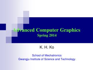
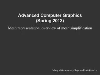
Advanced Computer Graphics (Spring 2013). CS 283, Lecture 10: Monte Carlo Integration Ravi Ramamoorthi http:// inst.eecs.berkeley.edu /~cs283 /sp13. Acknowledgements and many slides courtesy: Thomas Funkhouser, Szymon Rusinkiewicz and Pat Hanrahan. Motivation.

E N D
Advanced Computer Graphics (Spring 2013) CS 283, Lecture 10: Monte Carlo Integration Ravi Ramamoorthi http://inst.eecs.berkeley.edu/~cs283/sp13 Acknowledgements and many slides courtesy: Thomas Funkhouser, Szymon Rusinkiewicz and Pat Hanrahan
Motivation Rendering = integration • Reflectance equation: Integrate over incident illumination • Rendering equation: Integral equation Many sophisticated shading effects involve integrals • Antialiasing • Soft shadows • Indirect illumination • Caustics
Monte Carlo • Algorithms based on statistical sampling and random numbers • Coined in the beginning of 1940s. Originally used for neutron transport, nuclear simulations • Von Neumann, Ulam, Metropolis, … • Canonical example: 1D integral done numerically • Choose a set of random points to evaluate function, and then average (expectation or statistical average)
Monte Carlo Algorithms Advantages • Robust for complex integrals in computer graphics (irregular domains, shadow discontinuities and so on) • Efficient for high dimensional integrals (common in graphics: time, light source directions, and so on) • Quite simple to implement • Work for general scenes, surfaces • Easy to reason about (but care taken re statistical bias) Disadvantages • Noisy • Slow (many samples needed for convergence) • Not used if alternative analytic approaches exist (but those are rare)
Outline • Motivation • Overview, 1D integration • Basic probability and sampling • Monte Carlo estimation of integrals
Integration in 1D f(x) x=1 Slide courtesy of Peter Shirley
We can approximate • Standard integration methods like trapezoidal • rule and Simpsons rule • Advantages: • Converges fast for smooth integrands • Deterministic • Disadvantages: • Exponential complexity in many dimensions • Not rapid convergence for discontinuities g(x) f(x) x=1 Slide courtesy of Peter Shirley
Or we can average f(x) E(f(x)) x=1 Slide courtesy of Peter Shirley
Estimating the average • Monte Carlo methods (random choose samples) • Advantages: • Robust for discontinuities • Converges reasonably for large dimensions • Can handle complex geometry, integrals • Relatively simple to implement, reason about f(x) E(f(x)) x1 xN Slide courtesy of Peter Shirley
Other Domains f(x) < f >ab x=a x=b Slide courtesy of Peter Shirley
Eye Pixel x Surface Multidimensional Domains Same ideas apply for integration over … • Pixel areas • Surfaces • Projected areas • Directions • Camera apertures • Time • Paths
Outline • Motivation • Overview, 1D integration • Basic probability and sampling • Monte Carlo estimation of integrals
Random Variables • Describes possible outcomes of an experiment • In discrete case, e.g. value of a dice roll [x = 1-6] • Probability p associated with each x (1/6 for dice) • Continuous case is obvious extension
Expected Value • Expectation • For Dice example:
Sampling Techniques Problem: how do we generate random points/directions during path tracing? • Non-rectilinear domains • Importance (BRDF) • Stratified Eye x Surface
Generating Random Points Uniform distribution: • Use random number generator 1 Probability 0 W
Generating Random Points Specific probability distribution: • Function inversion • Rejection • Metropolis 1 Probability 0 W
Common Operations Want to sample probability distributions • Draw samples distributed according to probability • Useful for integration, picking important regions, etc. Common distributions • Disk or circle • Uniform • Upper hemisphere for visibility • Area luminaire • Complex lighting like an environment map • Complex reflectance like a BRDF
1 CumulativeProbability 0 W Generating Random Points
1 x x x x x x x Probability x x x 0 W Rejection Sampling
Outline • Motivation • Overview, 1D integration • Basic probability and sampling • Monte Carlo estimation of integrals
Monte Carlo Path Tracing Big diffuse light source, 20 minutes Motivation for rendering in graphics: Covered in detail in next lecture Jensen
Monte Carlo Path Tracing 1000 paths/pixel Jensen
Estimating the average • Monte Carlo methods (random choose samples) • Advantages: • Robust for discontinuities • Converges reasonably for large dimensions • Can handle complex geometry, integrals • Relatively simple to implement, reason about f(x) E(f(x)) x1 xN Slide courtesy of Peter Shirley
Other Domains f(x) < f >ab x=a x=b Slide courtesy of Peter Shirley
Variance E(f(x)) x1 xN
Variance for Dice Example? • Work out on board (variance for single dice roll)
Variance Variance decreases as 1/N Error decreases as 1/sqrt(N) E(f(x)) x1 xN
Variance • Problem: variance decreases with 1/N • Increasing # samples removes noise slowly E(f(x)) x1 xN
Variance Reduction Techniques • Importance sampling • Stratified sampling
Importance Sampling Put more samples where f(x) is bigger E(f(x)) x1 xN
Importance Sampling • This is still unbiased E(f(x)) for all N x1 xN
Importance Sampling • Zero variance if p(x) ~ f(x) E(f(x)) Less variance with better importance sampling x1 xN
Stratified Sampling • Estimate subdomains separately Arvo Ek(f(x)) x1 xN
Stratified Sampling • This is still unbiased Ek(f(x)) x1 xN
Stratified Sampling • Less overall variance if less variance in subdomains Ek(f(x)) x1 xN