Download
1 / 41
410 likes | 571 Vues
2. Cosmologia Despues de WMAP. Menu du Jour. Historia del descubrimiento del CMB Fisica del CMB - Radiacion de Cuerpo negro T=2.73 K - Dipolo (Doppler) - Fluctuaciones - Espectro de Potencia Angular 3. Observaciones - COBE y WMAP

E N D
Menu du Jour • Historia del descubrimiento del CMB • Fisica del CMB • - Radiacion de Cuerpo negro T=2.73 K • - Dipolo (Doppler) • - Fluctuaciones • - Espectro de Potencia Angular • 3. Observaciones • - COBE y WMAP • 4. Corroboracion del dipolo: velocidades peculiares • 5. Parametros cosmologicos: lo que sabemos hoy
CMB Dipole DT = 3.358 mK V_sun w.r.t CMB: 369 km/s towards l=264o , b=+48o Motion of the Local Group: V = 627 km/s towards l = 276o b= +30o
Removing the Galactic Contamination: see QuickTime movie mw in cosmology2
Qualitative Description of the CMB Power Spectrum • As long as matter is ionized, baryons and photons are coupled via • Thomson scattering: we refer to a “photon-baryon fluid” • Photons provide the pressure of the fluid, while baryons provide • the mass density, i.e. the inertia. • Gravity tries to compress the fluid, while pressure resists it: • acoustic oscillations are set. • The Universe reaches the epoch of recombination with density • fluctuations (of amplitude of ~1 part in 100,000). • Acoustic oscillations take place within the potential wells of the • density fluctuations: the compression phase of the oscillation • produces a slight enhancement in temperature of the fluid, • the rarefaction phase produces temperature decrement. • As the Universe recombines, the coupling between baryons and • photons ceases, and the two components separate. The photon • fluid ceases to oscillate and the temperature fluctuations “freeze” • at the epoch of last scattering. • The physical scale of the fluctuations at that epoch translates into • an angle, as seen from our vantage point at z=0: the larger the physical • scale, the larger the angle. [Visit the website of Wayne Hu: http://background.uchicago.edu/~whu]
Qualitative Description of the CMB Power Spectrum • The map of CMB • T fluctuations is • analyzed in terms • of its spherical • harmonics. • The eigennumber l • is inversely prop. • to the angular scale: • a = 100o / l • A fluctuation of • comoving physical • size l Mpc at the • epoch of recombination • subtends an angle • a ~ 17” l • in the sky at the • present time. Image credit: W. Hu
Qualitative Description of the CMB Power Spectrum At any given time before recombination, the largest l possible for an acoustic mode is that which the sound speed can travel in the Hubble time • At recombination (z~1000), the Hubble • radius is about 370,000 l.y., which • translates into a comoving distance of • ~ 100 Mpc, i.e. an angle a ~ 1700”, or half a degree. The acoustic mode that had time to compress ( heat) the fluid for the first time at z~1000 should thus have an angular size of half a degree. “Frozen” by decoupling, that mode should appear as a peak at l = 100/a ~ 200
Qualitative Description of the CMB Power Spectrum By analogous logic, the next acoustic mode should correspond to an oscillation that had time to compress and expand once: its angular scale should thus be half that of the fundamental mode. The second mode is a rarefaction mode. The third mode is one that went through the cycle: compression-rarefaction-compression in one Hubble time; its angular scale is 1/3 that of the fundamental mode and it is caught at z~1000 near max compression. And so on.
Dependence of power spectrum on W The position ( l number) of the peaks of the power spectrum is strongly dependent on the curvature of space. The identification of the first acoustic peak indicated that the Universe is spatially FLAT. Display curvature2 Quick Time Movie in cosmology2
Variations in the CMB Power Spectrum Varying h between 0.35 and 0.7 h2Wb = 0.0125 is fixed Varying Wb between 0.01 and 0.10 h = 0.5 is fixed Increasing the baryon density increases the density of the coupled photon-baryon fluid, altering the balance between pressure and gravity in the fuid. Compression modes (peaks 1 and 3) are enhanced with respect to rarefaction modes (peak 2). the relative height of contiguous peaks yields Wb Credit: Martin White
Varying L between 0 and 0.9 h2Wb = 0.0125 and h=0.5 are fixed Time variation of the CMB power spectrum between a(t)=1/2000 and a(t)=1 (now) The angle subtended by a given physical size at last scattering (i.e. a given mode) decreases as the Universe expands, shifting the peaks to the right (high l, small angle).
CMB Power Spectrum according to WMAP
The Sunyaev-Zel’dovich Effect
Recovering the LG motion from Galaxy Surveys • The Luminosity-Linewidth relation • Its Calibration and the Determination of Ho • Convergence Depth of the Local Universe • The Local Group reflex motion
Measurement of a velocity Width 1. Get good image of galaxy, measure PA, position slit 2. Pick spectral line, measure peak l along slit 3. Center kinematically 4. Fold about kinematical center 5. Correct for disk inclination, using isophotal ellipticity Outer slope 6. You now have a rotation curve. Pick a parametric model and fit it. E.g. Inner scale length
TF Relation: Data h= H/100 “Direct” slope is –7.6 “Inverse” slope is –7.8 SCI : cluster Sc sample …which is similar to the explicit theory-derived dependencea = 3 I band, 24 clusters, 782 galaxies [Giovanelli et al. 1997] a [WhereL a (rot. vel.) ]
Measuring the Hubble Constant A TF template relation is derived independently on the value of Ho . It can be derived for, or averaged over, a large number of galaxies, regions or environments. When calibrators are included, the Hubble constant can be gauged over the volume sampled by the template. From a selected sample of Cepheid Calibrators, Giovanelli et al. (1997) obtain H_not = 69+/-6 (km/s)/Mpc averaged over a volume of cz = 9500 km/s radius. The HST key-project team [Sakai et al 2000] gets 71+/-4+/-7
TF and the Peculiar Velocity Field • Given a TF template relation, the peculiar velocity of a galaxy can be derived from its offset Dm from that template, via • For a TF scatter of 0.35 mag, the error on the peculiar velocity of a single galaxy is typically (0.15-0.20) cz • For clusters, the error can be reduced by a factor if N galaxies per cluster are observed
No local Hubble Bubble Zehavi et al. (1999) : Local Hubble bubble within cz = 7500 km/s ? Giovanelli et al. (1999) :No local Hubble Bubble to cz ~ 15000 km/s
Convergence Depth Given a field of density fluctuations d(r) , an observer at r=0 will have a peculiar velocity: where W is W_mass The contribution to by fluctuations in the shell , asymptotically tends to zero as The cumulative by all fluctuations Within R thus exhibits the behavior : If the observer is the LG, the asymptotic matches the CMB dipole
The Peculiar Velocity Field to cz=6500 km/s SFI [Haynes et al 2000a,b] Peculiar Velocities in the LG reference frame
The Peculiar Velocity Field to cz=6500 km/s SFI [Haynes et al 2000a,b] Peculiar Velocities in the CMB reference frame
The Dipole of the Peculiar Velocity Field The reflex motion of the LG, w.r.t. field galaxies in shells of progressively increasing radius, shows : convergence with the CMB dipole, both in amplitude and direction, near cz ~ 5000 km/s. [Giovanelli et al. 1998] [Giovanelli et al. 2000]
Pacific Ocean Verrazzano Bias Map by Gerolamo da Verrazzano (1529)
The Dipole of the Peculiar Velocity Field Convergence to the CMB dipole is confirmed by the LG motion w.r.t. a set of 79 clusters out to cz ~ 20,000 km/s [Giovanelli et al 1999 ; Dale et al. 1999]