Download
1 / 46
690 likes | 1.97k Vues
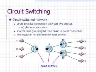
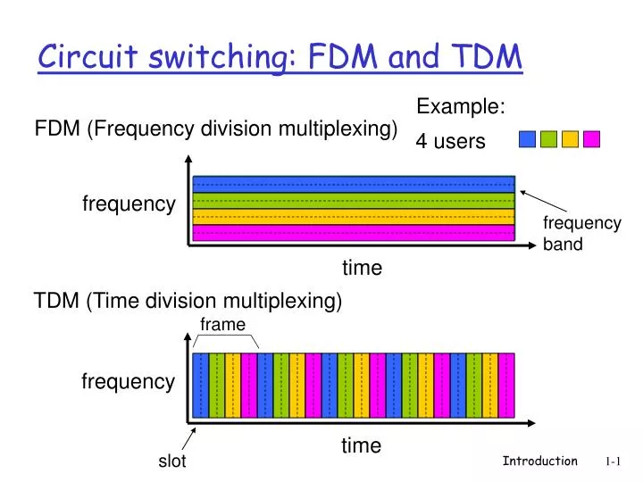
Example:. 4 users. FDM (Frequency division multiplexing). frequency. time. TDM (Time division multiplexing). frequency. time. Circuit switching: FDM and TDM. frequency band. frame. slot. Exercise.

E N D
Example: 4 users FDM (Frequency division multiplexing) frequency time TDM (Time division multiplexing) frequency time Circuit switching: FDM and TDM frequency band frame slot Introduction
Exercise • How long does it take to send a file of 640,000 bits from host A to host B over a circuit-switched network? • All links are 1.536 Mbps (in the whole freq. range) • Each link uses TDM with 24 slots/sec • 500 msec to establish end-to-end circuit Introduction
Exercise • How long does it take to send a file of 640,000 bits from host A to host B over a circuit-switched network? • All links are 1.536 Mbps (in the whole freq. range) • Each link uses FDM with 24 channels/frequency band • 500 msec to establish end-to-end circuit Introduction
user A, B packets share network resources each packet uses full link bandwidth resources used as needed Bandwidth division into “pieces” Dedicated allocation Resource reservation Network Core: Packet switching Resource contention: • aggregate resource demand can exceed amount available • congestion: packets queue, wait for link use, may get lost when queue fills • store and forward: packets move one hop at a time • Node receives complete packet before forwarding Each end-end data stream divided into packets Introduction
Takes L/R seconds to transmit (push out) packet of L bits on to link or R bps Entire packet must arrive at router before it can be transmitted on next link: store and forward Delay on 3 links = 3L/R (assuming zero propagation delay) Example: L = 7.5 Mbits R = 1.5 Mbps delay = 15 sec Delay of store-and-forward L R R R Introduction
Sequence of A & B packets does not have fixed pattern, shared on demand statistical multiplexing. TDM: each host gets same slot in revolving TDM frame. D E Statistical multiplexing 10 Mb/s Ethernet C A statistical multiplexing 1.5 Mb/s B queue of packets waiting for output link Introduction
1 Mb/s link Each user: 100 kb/s when “active” active 10% of time circuit-switching: 10 users packet switching: With 35 users, p(#active>10) < 0.0004 Packet switching allows more users to use network! Packet switching vs circuit switching N users 1 Mbps link Q: How did we get value 0.0004? Introduction
Packet switching vs circuit switching p(#active = n) p(#active n) Introduction
Packet switching is great for bursty data Resource sharing Simple, no call setup Packet switching problem:Excessive congestion leading to packet delay and loss Protocols needed for reliable data transfer, congestion control Circuit switching is good for guaranteed-quality services but expensive Sending video over the network Packet switching vs circuit switching Introduction
How do routers know how to get from A to B? They keep tables showing them the next hop neighbor on that route Datagram network: Destination address in packet determines next hop Router tables contain destination nexthop maps Routes may change during session Virtual circuit network: Each packet carries tag (virtual circuit ID – VC ID), one tag per “call” Router tables contain VC ID nexthop maps Fixed path determined at call setup time, remains fixed thru call Packet-switched networks: forwarding Introduction
VC tables are smaller and faster to search Only active calls on local links Datagram forwarding can handle route changes easier No per-call state in routers Datagram vs virtual circuit Introduction
Packet-switched networks Circuit-switched networks FDM TDM Datagram Networks Networks with VCs Network taxonomy Telecommunication networks • Datagram network is not either connection-oriented • or connectionless. • Internet provides both connection-oriented (TCP) and • connectionless services (UDP) to apps. Introduction
How to connect end systems to edge router? Residential access nets Institutional access networks (school, company) Mobile access networks Access network’s features: Bandwidth (bits per second) Shared or dedicated? Access networks Introduction
Dialup via modem Up to 56Kbps direct access to router (often less) Can’t surf and phone at same time: can’t be “always on” Residential access dedicated access • ADSL: asymmetric digital subscriber line • Up to 1 Mbps upstream (today typically < 256 kbps) • Up to 8 Mbps downstream (today typically < 1 Mbps) • FDM on phone line for upstream, downstream and voice sharedaccess • HFC: hybrid fiber coaxial cable • Asymmetric: up to 30Mbps downstream, 2 Mbps upstream • Network of cable and fiber attaches homes to ISP router • Homes share access to router Introduction
Company/university local area network (LAN) connects end system to edge router Ethernet: Shared or dedicated link connects end system and router 10 Mbs, 100Mbps, Gigabit Ethernet Company access: local area networks Introduction
Shared wireless access network connects end system to router Via base station aka “access point” Wireless LANs: 802.11b (WiFi): 11 Mbps Wider-area wireless access Connect to them via WAP phones Provided by telco operator Popular in Europe and Japan router base station mobile hosts Wireless access networks Introduction
Typical home network components: ADSL or cable modem Router/firewall/NAT Ethernet Wireless access point Home networks wireless laptops to/from cable headend cable modem router/ firewall wireless access point Ethernet Introduction
Roughly hierarchical At center: “tier-1” ISPs (e.g., MCI, Sprint, AT&T), national/international coverage Treat each other as equals NAP Tier-1 providers also interconnect at public network access points (NAPs) Tier-1 providers interconnect (peer) privately Internet structure Tier 1 ISP Tier 1 ISP Tier 1 ISP Introduction
Seattle POP: point-of-presence DS3 (45 Mbps) OC3 (155 Mbps) OC12 (622 Mbps) OC48 (2.4 Gbps) Tacoma to/from backbone peering New York … …. Stockton Cheyenne Chicago Pennsauken Relay Wash. DC San Jose Roachdale Kansas City … … … Anaheim to/from customers Atlanta Fort Worth Orlando Tier-1 ISP: Sprint Sprint US backbone network Introduction
“Tier-2” ISPs: smaller (often regional) ISPs Connect to one or more tier-1 ISPs, possibly other tier-2 ISPs NAP Tier-2 ISPs also peer privately with each other, interconnect at NAP Tier-2 ISP pays tier-1 ISP for connectivity to rest of Internet Tier-2 ISP is customer of tier-1 provider Tier-2 ISP Tier-2 ISP Tier-2 ISP Tier-2 ISP Tier-2 ISP Internet structure Tier 1 ISP Tier 1 ISP Tier 1 ISP Introduction
“Tier-3” ISPs and local ISPs Last hop (“access”) network (closest to end systems) Tier 3 ISP local ISP local ISP local ISP local ISP local ISP local ISP local ISP local ISP NAP Local and tier- 3 ISPs are customers of higher tier ISPs connecting them to rest of Internet Tier-2 ISP Tier-2 ISP Tier-2 ISP Tier-2 ISP Tier-2 ISP Internet structure Tier 1 ISP Tier 1 ISP Tier 1 ISP Introduction
Two networks can have Customer-provider relationship – provider sells access to customer Peer-peer relationship – networks can reach each others’ customers at no charge Networks peer if they have same size/status Internet structure Introduction
A packet passes through many networks! Tier 3 ISP local ISP local ISP local ISP local ISP local ISP local ISP local ISP local ISP NAP Tier-2 ISP Tier-2 ISP Tier-2 ISP Tier-2 ISP Tier-2 ISP Internet structure Tier 1 ISP Tier 1 ISP Tier 1 ISP Introduction
Packets queue in router buffers Packet arrival rate to link exceeds output link capacity Packets queue, wait for turn If queue is full, packets are dropped packet being transmitted (delay) packets queueing (delay) free (available) buffers: arriving packets dropped (loss) if no free buffers How do loss and delay occur? A B Introduction
1. processing: Check bit errors Determine output link transmission A propagation B nodal processing queueing Four sources of packet delay 2. queueing • Time waiting at output link for transmission • Depends on congestion level of router Introduction
3. Transmission delay: R=link bandwidth (bps) L=packet length (bits) time to send bits into link = L/R 4. Propagation delay: d = length of physical link s = propagation speed in medium (~2x10⁸ m/sec) propagation delay = d/s transmission A propagation B nodal processing queueing Four sources of packet delay Note: s and R are very different quantities! Introduction
Cars “propagate” at 100 km/hr Toll booth takes 12 sec to service a car (transmission time) car~bit; caravan ~ packet Q: How long until the whole caravan is lined up before 2nd toll booth? Time to “push” entire caravan through toll booth onto highway = 12*10 = 120 sec Time for last car to propagate from 1st to 2nd toll both: 100km/(100km/hr)= 1 hr A: 62 minutes toll booth toll booth Caravan analogy 100 km 100 km 10-car caravan Introduction
Cars now “propagate” at 1000 km/hr Toll booth now takes 1 min to service a car Q:Will cars arrive to 2nd booth before all cars serviced at 1st booth? Yes! After 7 min, 1st car at 2nd booth and 3 cars still at 1st booth. 1st bit of packet can arrive at 2nd router before packet is fully transmitted at 1st router! toll booth toll booth Caravan analogy (more) 100 km 100 km 10-car caravan Introduction
Nodal delay • dproc = processing delay • typically a few microsecs or less • dqueue = queuing delay • depends on congestion • dtrans = transmission delay • = L/R, significant for low-speed links • dprop = propagation delay • a few microsecs to hundreds of msecs Introduction
R=link bandwidth (bps) L=packet length (bits) a=average packet arrival rate Queueing delay (revisited) traffic intensity = La/R • L*a/R ~ 0: average queueing delay small • L*a/R -> 1: delays become large • L*a/R > 1: more “work” arriving than can be serviced, average delay infinite! Introduction
“Real” Internet delays and routes • What do “real” Internet delay & loss look like? • Traceroute program: provides delay measurement from source to router along end-end Internet path towards destination. For all i: • Sends three packets that will reach router i on path towards destination • Router i will return packets to sender • Sender times interval between transmission and reply. 3 probes 3 probes 3 probes Introduction
“Real” Internet delays and routes traceroute: gaia.cs.umass.edu to www.eurecom.fr Three delay measurements from gaia.cs.umass.edu to cs-gw.cs.umass.edu 1 cs-gw (128.119.240.254) 1 ms 1 ms 2 ms 2 border1-rt-fa5-1-0.gw.umass.edu (128.119.3.145) 1 ms 1 ms 2 ms 3 cht-vbns.gw.umass.edu (128.119.3.130) 6 ms 5 ms 5 ms 4 jn1-at1-0-0-19.wor.vbns.net (204.147.132.129) 16 ms 11 ms 13 ms 5 jn1-so7-0-0-0.wae.vbns.net (204.147.136.136) 21 ms 18 ms 18 ms 6 abilene-vbns.abilene.ucaid.edu (198.32.11.9) 22 ms 18 ms 22 ms 7 nycm-wash.abilene.ucaid.edu (198.32.8.46) 22 ms 22 ms 22 ms 8 62.40.103.253 (62.40.103.253) 104 ms 109 ms 106 ms 9 de2-1.de1.de.geant.net (62.40.96.129) 109 ms 102 ms 104 ms 10 de.fr1.fr.geant.net (62.40.96.50) 113 ms 121 ms 114 ms 11 renater-gw.fr1.fr.geant.net (62.40.103.54) 112 ms 114 ms 112 ms 12 nio-n2.cssi.renater.fr (193.51.206.13) 111 ms 114 ms 116 ms 13 nice.cssi.renater.fr (195.220.98.102) 123 ms 125 ms 124 ms 14 r3t2-nice.cssi.renater.fr (195.220.98.110) 126 ms 126 ms 124 ms 15 eurecom-valbonne.r3t2.ft.net (193.48.50.54) 135 ms 128 ms 133 ms 16 194.214.211.25 (194.214.211.25) 126 ms 128 ms 126 ms 17 * * * 18 * * * 19 fantasia.eurecom.fr (193.55.113.142) 132 ms 128 ms 136ms trans-oceanic link * means no response (probe lost, router not replying) Introduction
Packet loss • Queue (aka buffer) preceding link in buffer has finite capacity • When packet arrives to full queue, packet is dropped (aka lost) • Lost packet may be retransmitted by previous node, by source end system, or not retransmitted at all Introduction
Networks are complex! many “pieces”: hosts routers links of various media applications protocols hardware, software Question: Is there any hope of organizing structure of network? Or at least our discussion of networks? Protocol “Layers” Introduction
ticket (complain) baggage (claim) gates (unload) runway landing airplane routing ticket (purchase) baggage (check) gates (load) runway takeoff airplane routing airplane routing Organization of air travel a series of steps Introduction
ticket ticket (purchase) baggage (check) gates (load) runway (takeoff) airplane routing ticket (complain) baggage (claim gates (unload) runway (land) airplane routing baggage gate airplane routing airplane routing takeoff/landing airplane routing departure airport intermediate air-traffic control centers arrival airport Layering of airline functionality Layers:each layer implements a service • via its own internal-layer actions • relying on services provided by layer below Introduction
Why layering? Dealing with complex systems: • Explicit structure allows identification, relationship of complex system’s pieces • Modularization eases maintenance, updating of system • Change of implementation of layer’s service transparent to rest of system • e.g., change in gate procedure doesn’t affect rest of system Introduction
Application: supporting network applications FTP, SMTP, HTTP Transport: host-host data transfer TCP, UDP Network: routing of datagrams from source to destination IP, routing protocols Link: data transfer between neighboring network elements PPP, Ethernet Physical: bits “on the wire” application transport network link physical Internet protocol stack Introduction
Link layer vs. network layer IP 1.2.3.4 Link protocol will deliver a message to the right device in local network LA4 LA5 LA1 LA3 LA6 workstation A router 1 LA8 LA7 LA2 LA9 router 2 workstation C IP 7.8.9.10 IP 1.2.3.5 EthernetShared link medium Network protocol will help us deliver a messagefrom source to destination via routerswho know the nexthop from their routing table LA10 server B Introduction
How to talk on the Internet? workstation A router 1 link layer – link protocol router 2 This is a message for router 1 network layer – IP protocol This is message from A to B router 3 transport layer – TCP/UDP/… protocol This is message 2 for Web application server B application layer – HTTP protocol I want this webpage! Introduction
network link physical link physical M M Ht Ht M M Hn Hn Hn Hn Ht Ht Ht Ht M M M M Hl Hl Hl Hl Hl Hl Hn Hn Hn Hn Hn Hn Ht Ht Ht Ht Ht Ht M M M M M M source Encapsulation message application transport network link physical segment datagram frame switch destination application transport network link physical router Introduction
1961: Kleinrock - queueing theory shows effectiveness of packet-switching 1964: Baran - packet-switching in military nets 1967: ARPAnet conceived by Advanced Research Projects Agency 1969: first ARPAnet node operational 1972: ARPAnet public demonstration NCP (Network Control Protocol) first host-host protocol first e-mail program ARPAnet has 15 nodes Internet History 1961-1972: Early packet-switching principles Introduction
1970: ALOHAnet satellite network in Hawaii 1974: Cerf and Kahn - architecture for interconnecting networks 1976: Ethernet at Xerox PARC late70’s: proprietary architectures: DECnet, SNA, XNA late 70’s: switching fixed length packets (ATM precursor) 1979: ARPAnet has 200 nodes Cerf and Kahn’s internetworking principles: minimalism, autonomy - no internal changes required to interconnect networks best effort service model stateless routers decentralized control define today’s Internet architecture Internet History 1972-1980: Internetworking, new and proprietary nets Introduction
1983: deployment of TCP/IP 1982: smtp e-mail protocol defined 1983: DNS defined for name-to-IP-address translation 1985: ftp protocol defined 1988: TCP congestion control New national networks: Csnet, BITnet, NSFnet, Minitel 100,000 hosts connected to confederation of networks Internet History 1980-1990: new protocols, a proliferation of networks Introduction
Early 1990’s: ARPAnet decommissioned 1991: NSF lifts restrictions on commercial use of NSFnet (decommissioned, 1995) early 1990s: Web Hypertext [Bush 1945, Nelson 1960’s] HTML, HTTP: Berners-Lee 1994: Mosaic, later Netscape Late 1990’s: commercialization of the Web Late 1990’s – 2000’s: More killer apps: instant messaging, P2P file sharing Network security to forefront Est. 50 million host, 100 million+ users Backbone links running at Gbps Internet History 1990, 2000’s: commercialization, the Web, new apps Introduction