Download
1 / 57
580 likes | 810 Vues
Price Levels and the Exchange Rate in the Long Run. Lecture Notes on Ch. 15 of Krugman and Obstfeld, 7 th Ed. Udayan Roy, December 2008. Purchasing Power Parity. The simplest theory of prices and exchange rates for the long run is (absolute) purchasing power parity. The Real Exchange Rate.

E N D
Price Levels and the Exchange Rate in the Long Run Lecture Notes on Ch. 15 of Krugman and Obstfeld, 7th Ed. Udayan Roy, December 2008
Purchasing Power Parity • The simplest theory of prices and exchange rates for the long run is (absolute) purchasing power parity.
The Real Exchange Rate • Let us consider the price of an iPod in US and Europe: • In US, it is PUS = $200 • In Europe, it is PE = €150 • The value of the euro is E = 2 dollars per euro • So, Europe's price in dollars is E × PE = $300 • So, each iPod in Europe costs as much as 1.5 iPods in US • E × PE / PUS= 1.5 • This is the Real dollar/euro Exchange Rate for iPods
The Real Exchange Rate • In general, the real exchange rate is a broad summary measure of the prices of one country’s goods and services relative to the other's. • The real dollar/euro exchange rate is the number of US reference commodity baskets—not just iPods—that one European reference commodity basket is worth: • Equation (15-6)
the real dollar/euro exchange rate • Example: If the European reference commodity basket costs €100, the U.S. basket costs $120, and the nominal exchange rate is $1.20 per euro, then the real dollar/euro exchange rate (q$/€) is 1 U.S. basket per European basket.
Real depreciation and appreciation • Real depreciation of the dollar against the euro • A rise in the real dollar/euro exchange rate (q$/€↑) • is a fall in the purchasing power of a dollar within Europe’s borders relative to its purchasing power within the United States • Or alternatively, a fall in the purchasing power of America’s products in general over Europe’s. • Real appreciation of the dollar against the euro is the opposite of a real depreciation: a fall in q$/€.
Absolute PPP • A very simple theory of the real exchange rate (called Absolute Purchasing Power Parity) says that: q = 1 • Why?
Law of one price • Going back for a second to the iPod example, one can argue that PUS, the dollar price in the US, ought to be equal to E × PE, the dollar price in Europe. That is, • E × PE = PUS. • In general, E$/€ x PE = PUS. • Therefore, q$/€ = (E$/€ x PE)/PUS = 1. • This is the Law of One Price or Absolute Purchasing Power Parity.
Absolute PPP: logical but not factual • Despite the logical appeal of Absolute Purchasing Power Parity, available data suggests that it is not true • We need to look for another theory of the real exchange rate, q.
A different theory of q: Ch 16 • In search of a more useful theory of the real exchange rate, we briefly skip ahead to Chapter 16 • That chapter is about the short run. • But parts of it can help us study the long run as well
Determinants of Aggregate Demand • Aggregate demand (D) is the aggregate amount of goods and services that people are willing to buy. • It consists of the following types of expenditure: • consumption expenditure (C) • investment expenditure (I) • government purchases (G) • net expenditure by foreigners: the current account (CA)
Determinants of Aggregate Demand • Consumption expenditure (C) depends on Disposable income (Y-T), which is income (Y) minus taxes (T). • More disposable income means more consumption expenditure • But consumption typically increases less than the amount by which disposable income increases. • Real interest rates may influence the amount of saving and consumption, but we assume that they are relatively unimportant here. • Wealth may also influence consumption, but we assume that it is relatively unimportant here.
Determinants of Aggregate Demand • The current account (CA) depends on: • Real exchange rate (q), which is the price of foreign products relative to the price of domestic products, both measured in domestic currency: q = EP*/P • As q rises, expenditure on domestic products rises and expenditure on foreign products falls. Therefore, when q rises, CA rises as well. • Disposable income: more disposable income (Y-T) means more expenditure on foreign products (imports). Therefore, when Y-T rises, CA falls.
Determinants of Aggregate Demand • Determinants of the current account include: • Real exchange rate: an increase in the real exchange rate increases the current account. • Disposable income: an increase in the disposable income decreases the current account.
Current account depends on the real exchange rate and disposable income. Consumption depends on disposable income Investment and government purchases, both exogenous Determinants of Aggregate Demand (cont.) • Aggregate demand is therefore expressed as: D = C(Y – T) + I + G + CA(q, Y – T) • Or more simply: D = D(q, Y – T, I, G)
Aggregate demand as a function of the real exchange rate, disposable income, investment, government purchases Value of output, income from production Short Run Equilibrium for Aggregate Demand and Output • Equilibrium is achieved when the value of output Y equals aggregate demand D. Y = D(q, Y – T, I, G)
Output is greater than aggregate demand: firms decrease output Aggregate demand is greater than production: firms increase output Short Run Equilibrium for Aggregate Demand and Output (cont.) Y = D(q, Y – T, I, G)
Goods Market Equilibrium and the Real Exchange Rate: DD Schedule • How does the real exchange rate (q) affect the equilibrium of aggregate demand and output? • Therefore, a rise in the real exchange rate (q) makes foreign goods more expensive relative to domestic goods. • As a result, CA increases and, therefore, D increases. That is, D increases when q increases. • In equilibrium, Y = D. Therefore, Y increases when q increases. • This gives the DD curve. Y = D(q, Y – T, I, G)
Aggregate Demand, D 45° line The DD Curve Aggregate Demand (q2) Aggregate Demand (q1) • As q, the price of foreign goods, increases • Aggregate demand for domestic goods increases • Therefore, equilibrium output also increases • This gives us the DD curve Y2 Output, Y Y1 Real Exchange Rate, q DD Curve q2 q1 Output, Y Y2 Y1 Y = D(q, Y – T, I, G)
Long-Run Output • In the long run, output equals potential output • In the short run, which we will discuss in chapter 16, recessions can happen • During recessions, labor and other resources may remain unemployed and output may fall below the potential level • But in the long run markets for labor and other resources are assumed to function normally and to make supply equal to demand, thereby making unemployment impossible • Potential output is also called full-employment, and is denoted Yp. • In the long run, Y = Yp.
Long-Run Output • Full-employment output (Yp) increases when • The availability of labor increases • The quality of labor (human capital) increases • The availability of physical capital (equipment, structures, infrastructure) increases • The technology improves • Economic policies and institutions favor productive activity
Real Exchange Rate: long run • The DD curve tells us that • If the full-employment output is known, the long-run value of the real exchange rate can be obtained • If the full-employment output increases, so does the real exchange rate Real Exchange Rate, q DD Curve q2 q1 Output, Y Yp = Y2 Yp = Y1
Aggregate Demand, D 45° line Shifts of the DD Curve Aggregate Demand2 Aggregate Demand1 • Suppose the real exchange rate stays unchanged at q1. But • If either • Taxes (T) ↓ • Investment (I) or Government Purchases (G) ↑ • Worldwide preference for domestic goods ↑ • Or if some combination of the above happens • Then aggregate demand will increase and equilibrium output will increase even though q is unchanged • This implies that the DD curve will shift to the right Y2 Output, Y Y1 Real Exchange Rate, q DD1 DD2 q1 Output, Y Y2 Y1 Y = D(q, Y – T, I, G)
Real Exchange Rate: long run • Suppose Yp remains unchanged • If the DD curve shifts right, the real exchange rate decreases Real Exchange Rate, q DD1 DD2 q1 q2 Output, Y Yp
Real Exchange Rate: long run • Now we can list all the causes that make the real exchange rate decrease (q↓): • Domestic full-employment output (Yp)↓ • Demand for domestic output ↑ • Taxes (T) ↓ • Investment (I) or Government Purchases (G) ↑ • Worldwide preference for domestic goods ↑ • Domestic preference for foreign goods ↓ • Some combination of the above happens • Nothing else affects q
Real Exchange Rate: long run • Recall that the real exchange rate is the price of foreign goods • That is, q is the amount of domestic goods that one unit of foreign goods is worth • This price of foreign goods will decrease (q↓) if • Either the supply of domestic goods decreases (Yp↓) • Or the demand for domestic goods increases (T ↓, I↑, G↑, worldwide demand for domestic goods ↑)
The current account • Recall that CA = CA(q, Y – T) • Therefore, CA↑ if • I↓, G↓ • T↑, Yp↑ • Nothing else can affect the current account balance • Tariffs and other protectionist policies will not work! • CA = Yp – C(Yp – T) – G – I
Real Exchange Rate: long run • Note that our analysis of the real exchange rate has not even mentioned the money supply (Ms) • In the long run, changes in the supply of money or in the rate of growth of the supply of money have no effect on q
Money and Prices • We saw in the last chapter that any increase in the domestic money supply (Ms) leads to a proportional increase in the domestic price level (P). • Moreover, changes in the domestic money supply (Ms) cannot affect the foreign price level (P*) • And we have just seen that q = EP*/P is unaffected by any increase in Ms • Therefore, E must increase proportionally. • That is, in the long run, any increase in the domestic money supply (Ms) will cause a proportional increase in the value of the foreign currency (E).
Nominal and Real Exchange Rates in Long-Run Equilibrium • Note equations (15-6) and (15-7) above • The nominal dollar/euro exchange rate is • the real dollar/euro exchange rate times • the U.S.-Europe price level ratio.
Mathematics of growth rates • Consider three variables: x,y, and z … • … and their rates of growth: xg,yg, and zg. • Growth rates are computed as follows:xg = (xfuture – xnow) / xnow. • It can then be shown that • If z = x× y, then zg = xg+ yg • If z = x/ y, then zg = xg- yg • The same is true for expected growth rates, wherexge = (xfuturee – xnow) / xnow is the expected growth rate of x.
Exchange rates and inflation • Recall equation (15-7) • So, the results in the previous slide imply • Inflation is • expected inflation is • Then, we get equation (15-8)
Real interest rate parity • We start with interest rate parity • We end with real interest rate parity
Relative Purchasing Power Parity • I have discussed the various factors that can affect the real exchange rate (q) • However, I will assume that changes in q are isolated events and that there is no reason for people to expect continuous or sustained changes in q • That is, I will assume (qe–q)/q = 0 • This assumption is also called Relative Purchasing Power Parity (RPPP)
Exchange rates and inflation • Recall equation (15-8) • Under relative purchasing power parity, (qe–q)/q = 0. • Then, • see p. 376.
Purchasing Power Parity • Absolute PPP • Relative PPP
Exchange rates and inflation • According to Relative Purchasing Power Parity, • If the expected US inflation rate is 4% (eUS = 4) and Europe’s inflation rate is 7% (eE = 7), then the value of the euro will be expected to fall by 3%. • (Ee–E)/E = eUS–eE = 4 – 7 = – 3. • In short, whichever country has the higher expected inflation rate will face an expected loss in the value of its currency
Long-run effect of the growth rate of the money supply • We saw in Ch. 14 that in the long run any change inMg causes an identical change in . • I will assume that there are no other causes of inflation in the long run • In that case, one can write = Mg. • In the long run, inflation expectations are assumed to be, on average, accurate: e = . • So, when MgUS increases, both US andeUS increase by the same amount: e = = Mg.
Long-run effect of the growth rate of the money supply • R$ – R€ = (qe – q)/q + (eUS–eE)(15-9) • By relative PPP, R$ – R€ = eUS–eE • R$ – R€ = MgUS–eE. • R$ = R€ –eE + MgUS. • Therefore, in the long run, the domestic (nominal) interest rate can increase if (and only if) • The foreign real interest rate (R€ –eE) increases, or • The growth rate of the domestic money supply (MgUS) increases
The Fisher Effect • A rise (fall) in a country’s expected inflation rate will eventually cause an equal rise (fall) in the interest rate that deposits of its currency offer. • Figure 15-1 illustrates an example, where at time t0 the Federal Reserve unexpectedly increases the growth rate of the U.S. money supply to a higher level.
The Fisher Effect • In this example, the dollar interest rate rises because people expect more rapid future money supply growth and dollar depreciation. • The interest rate increase is associated with higher expected inflation and an immediate currency depreciation. • Figure 15-2 represents the main long-run prediction of the Fisher effect.
Figure 15-2: Inflation and Interest Rates in Switzerland, the United States, and Italy, 1970-2000
Long-run effect of the growth rate of the money supply • PUS = MUS/L(R$,YUS) (15-3) • The domestic price level increases if (and only if) • The domestic money supply (MUS) increases or • L(R$,YUS) decreases, which happens if • YUS decreases or • The domestic willingness to hold cash decreases or • R$increases, which happens if • the foreign real interest rate (R€ –eE) increases, or • the growth rate of the domestic money supply (MgUS) increases
Long-Run Nominal Exchange Rates • E$/€ = q$/€ x PUS/PE (15-6) • Therefore, the nominal exchange value of the foreign currency (E) increases if (and only if) • The foreign price level (PE) decreases • or, q increases, which happens if • Domestic full-employment output (Yf) ↑ • Demand for domestic output ↓ • Taxes (T) ↑ • Investment (I) or Government Purchases (G) ↓ • Worldwide preference for domestic goods ↓ • Domestic preference for foreign goods ↑ • or, the domestic price level (PUS) increases, which happens if • The domestic money supply (MUS) increases • Yf decreases or • The domestic willingness to hold cash decreases or • the foreign real interest rate (R€ –eE) increases, or • the growth rate of the domestic money supply (MgUS) increases Note that the effect of the domestic full-employment output on the exchange rate is ambiguous.
(a) U.S. money supply, MUS (b) Dollar interest rate, R$ R$2 = R$1 + Slope = + MUS, t0 R$1 Slope = t0 t0 Time Time (d) Dollar/euro exchange rate, E$/€ (c) U.S. price level, PUS Slope = + Slope = + Slope = Slope = t0 Time t0 Time Figure 15-1: Long-Run Time Paths of U.S. Economic Variables after a Permanent Increase in the Growth Rate of the U.S. Money Supply