Download
1 / 58
580 likes | 658 Vues
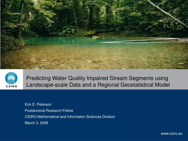
Predicting Water Quality Impaired Stream Segments using Landscape-scale Data and a Regional Geostatistical Model. Erin E. Peterson Postdoctoral Research Fellow CSIRO Mathematical and Information Sciences Division March 3, 2006. This research is funded by. This research is funded by.

E N D
Predicting Water Quality Impaired Stream Segments using Landscape-scale Data and a Regional Geostatistical Model Erin E. Peterson Postdoctoral Research Fellow CSIRO Mathematical and Information Sciences Division March 3, 2006
This research is funded by This research is funded by U.S.EPA U.S.EPA 凡 Science To Achieve Science To Achieve Results (STAR) Program Results (STAR) Program Cooperative Cooperative CR CR - - 829095 829095 # # Agreement Agreement Space-Time Aquatic Resources Modeling and Analysis Program The work reported here was developed under STAR Research Assistance Agreement CR-829095 awarded by the U.S. Environmental Protection Agency (EPA) to Colorado State University. This presentation has not been formally reviewed by EPA. EPA does not endorse any products or commercial services mentioned in this presentation.
Collaborators Dr. David M. Theobald Natural Resource Ecology Lab Department of Recreation & Tourism Colorado State University, USA Dr. N. Scott Urquhart Department of Statistics Colorado State University, USA Dr. Jay M. Ver Hoef National Marine Mammal Laboratory, Seattle, USA Andrew A. Merton Department of Statistics Colorado State University, USA
Overview Introduction ~ Background ~ Patterns of spatial autocorrelation in stream water chemistry ~ Visualizing model predictions ~ Current and future research in SEQ
Purpose of Our Research • Water Quality Monitoring Goals • Create a regional water quality assessment • Identify water quality impaired stream segments • Purpose • Demonstrate a geostatistical methodology based on • Coarse-scale GIS data • Field surveys • Predict water quality characteristics about stream segments throughout a region
How are geostatistical model different from traditional statistical models? • Traditional statistical models (non-spatial) • Residual error (ε) is assumed to be uncorrelated • ε = unexplained variability in the data • Geostatistical models • Residual errors are correlated through space • Spatial patterns in residual error resulting from unidentified process(es) • Model spatial structure in the residual error • Explain additional variability in the data • Generate predictions at unobserved sites
10 Sill Semivariance Nugget Range 0 1000 0 Separation Distance Geostatistical Modelling • Fit an autocovariance function to data • Describes relationship between observations based on separation distance • 3 Autocovariance Parameters • Nugget: variation between sites as separation distance approaches zero • Sill: delineated where semivariance asymptotes • Range: distance within which spatial autocorrelation occurs
B A C Distance Measures and Spatial Relationships • Straight Line Distance (SLD) • As the crow flies
B A C Distance Measures and Spatial Relationships • Symmetric Hydrologic Distance (SHD) • As the fish swims
B A C Distance Measures and Spatial Relationships • Weighted asymmetric hydrologic distance (WAHD) • As the water flows • Incorporate flow direction & flow volume Ver Hoef, J.M., Peterson, E.E., and Theobald, D.M. (2006) Spatial Statistical Models that Use Flow and Stream Distance, Environmental and Ecological Statistics, to appear.
B A C Distance Measures and Spatial Relationships • Challenge: • Spatial autocovariance models developed for SLD may not be valid for hydrologic distances • Covariance matrix is not positive definite
Flow Asymmetric Autocovariance Models for Stream Networks • Weighted asymmetric hydrologic distance (WAHD) • Developed by Jay Ver Hoef, National Marine Mammal Laboratory, Seattle, WA, USA • Moving average models • Incorporate flow volume, flow direction, and use hydrologic distance • Positive definite covariance matrices Ver Hoef, J.M., Peterson, E.E., and Theobald, D.M., Spatial Statistical Models that Use Flow and Stream Distance, Environmental and Ecological Statistics. In Press.
Objectives Evaluate 8 chemical response variables • pH measured in the lab (PHLAB) • Conductivity (COND) measured in the lab μmho/cm • Dissolved oxygen (DO) mg/l • Dissolved organic carbon (DOC) mg/l • Nitrate-nitrogen (NO3) mg/l • Sulfate (SO4) mg/l • Acid neutralizing capacity (ANC) μeq/l • Temperature (TEMP) °C Determine which distance measure is most appropriate • SLD, SHD, WAHD? • More than one? Find the range of spatial autocorrelation
Maryland Biological Stream Survey (MBSS) Data • Maryland Department of Natural Resources • Maryland, USA • 1995, 1996, 1997 • Stratified probability-based random survey design • 1st, 2nd, and 3rd order non-tidal streams • 955 sites • 881 sites after pre-processing • 17 interbasins
Maryland, USA Baltimore Annapolis Washington D.C. Chesapeake Bay Study Area
N Spatial Distribution of MBSS Data
2 1 3 1 2 3 1 2 3 SHD AHD SLD Functional Linkage of Watersheds and Streams (FLoWS) • Create data for geostatistical modelling • Calculate watershed covariates for each stream segment • Calculate separation distances between sites • SLD, SHD, Asymmetric hydrologic distance (AHD) • Calculate the spatial weights for the WAHD • Convert GIS data to a format compatible with statistics software • FLoWS website: http://www.nrel.colostate.edu/projects/starmap
Watershed Segment B Watershed Segment A • Calculate the PI of each upstream segment on segment directly downstream A B • Calculate the PI of one survey site on another site • Flow-connected sites • Multiply the segment PIs C Watershed Area A Segment PI of A = Watershed Area A+B Spatial Weights for WAHD • Proportional influence (PI):influence of each neighboring survey site on a downstream survey site • Weighted by catchment area: Surrogate for flow volume
Calculate the PI of each upstream segment on segment directly downstream A C B E D • Calculate the PI of one survey site on another site • Flow-connected sites • Multiply the segment PIs F G H Spatial Weights for WAHD • Proportional influence (PI):influence of each neighboring survey site on a downstream survey site • Weighted by catchment area: Surrogate for flow volume survey sites stream segment
Calculate the PI of each upstream segment on segment directly downstream • Calculate the PI of one survey site on another site • Flow-connected sites • Multiply the segment PIs Site PI = B * D * F * G Spatial Weights for WAHD • Proportional influence (PI):influence of each neighboring survey site on a downstream survey site • Weighted by catchment area: Surrogate for flow volume A C B E D F G H
Data for Geostatistical Modelling • Distance matrices • SLD, SHD, AHD • Spatial weights matrix • Contains flow dependent weights for WAHD • Watershed covariates • Lumped watershed covariates • Mean elevation, % Urban • Observations • MBSS survey sites
Geostatistical Modeling Methods • Validation Set • Unique for each chemical response variable • Initial Covariate Selection • 5 covariates • Model Development • Restricted model space to all possible linear models • 4 model sets
Log-likelihood function of the parameters ( ) given the observed data Z is: and Both maximum likelihood estimators can be written as functions of alone Derive the profile log-likelihood function by substituting the MLEs ( ) back into the log-likelihood function Geostatistical Modelling Methods Geostatistical model parameter estimation Maximize the profile log-likelihood function Maximizing the log-likelihood with respect to B and sigma2 yields:
where C1 is the correlation based on the distance between two sites, h, given the autocorrelationparameter estimates: nugget ( ), sill ( ), and range ( ). • Correlation matrix for WAHD model • Fit exponential autocorrelation function (C1) • Hadamard (element-wise) product of C1 & square root of spatial weights matrix forced into symmetry ( ) Geostatistical Modeling Methods Correlation matrix for SLD and SHD models Fit exponential autocorrelation function
Geostatistical Modeling Methods • Model selection within model set • GLM: Akaike Information Corrected Criterion (AICC) • Geostatistical models: Spatial AICC (Hoeting et al., in press) where n is the number of observations, p-1 is the number of covariates, and k is the number of autocorrelation parameters. http://www.stat.colostate.edu/~jah/papers/spavarsel.pdf • Model selection between model types • 100 Predictions: Universal kriging algorithm • Mean square prediction error (MSPE) • Cannot use AICC to compare models based on different distance measures • Model comparison • r2 for observed vs. predicted values
Summary statistics for distance measures in kilometers using DO (n=826). * Asymmetric hydrologic distance is not weighted here Results • Summary statistics for distance measures • Spatial neighborhood differs • Affects number of neighboring sites • Affects median, mean, and maximum separation distance
180.79 301.76 SLD SHD WAHD Results • Range of spatial autocorrelation differs • Shortest for SLD • TEMP = shortest range values • DO = largest range values Mean Range Values SLD = 28.2 km SHD = 88.03 km WAHD = 57.8 km
GLM SLD MSPE SHD WAHD Results • Distance Measures • GLM always has less predictive ability • More than one distance measure usually performed well • SLD, SHD, WAHD: PHLAB & DOC • SLD and SHD : ANC, DO, NO3 • WAHD & SHD: COND, TEMP • SLD distance: SO4
Predictive ability of models Strong: ANC, COND, DOC, NO3, PHLAB Weak: DO, TEMP, SO4 r2 r2 GLM SLD SHD WAHD Results
Distance measure influences how spatial relationships are represented in a stream network • Site’s relative influence on other sites • Dictates form and size of spatial neighborhood • Important because… • Impacts accuracy of the geostatistical model predictions SHD WAHD SLD Discussion
SLD, SHD, and WAHD represent spatial autocorrelation in continuous coarse-scale variables SLD • > 1 distance measure performed well • SLD never substantially inferior • Do not represent movement through network • Different range of spatial autocorrelation? • Larger SHD and WAHD range values • Separation distance larger when restricted to network SHD Discussion Patterns of spatial autocorrelation found at relatively coarse scale • Geostatistical models describe more variability than GLM
244 sites did not have neighbors Sample Size = 881 Number of sites with ≤1 neighbor: 393 Mean number of neighbors per site: 2.81 Frequency Number of Neighboring Sites Discussion • Probability-based random survey design (-) affected WAHD • Maximize spatial independence of sites • Does not represent spatial relationships in networks • Validation sites randomly selected
4500 WAHD GLM Difference (O – E) 0 0 1 2 3 4 5 6 7 9 10 11 12 13 14 15 16 17 8 Number of Neighboring Sites Discussion WAHD models explained more variability as neighboring sites increased • Not when neighbors had: • Similar watershed conditions • Significantly different chemical response values
4500 WAHD GLM Difference (O – E) 0 0 1 2 3 4 5 6 7 9 10 11 12 13 14 15 16 17 8 Number of Neighboring Sites Discussion • GLM predictions improved as number of neighbors increased • Clusters of sites in space have similar watershed conditions • Statistical regression pulled towards the cluster • GLM contained hidden spatial information • Explained additional variability in data with > neighbors
Coarse COND SO4 ANC PH NO3 DOC Scale of unknown influential processes TEMP DO Fine 0.5 0 1.0 r2 Predictive Ability of Geostatistical Models
Conclusions • Spatial autocorrelation exists in stream chemistry data at a relatively coarse scale • Geostatistical models improve the accuracy of water chemistry predictions • Patterns of spatial autocorrelation differ between chemical response variables • Ecological processes acting at different spatial scales affect conditions at the survey site • SLD is the most suitable distance measure in Maryland for these chemical response variablesat this time • Unsuitable survey designs • SHD: GIS processing time is prohibitive
Conclusions • Results are scale specific • Spatial patterns change with survey scale • Other patterns may emerge at shorter separation distances • 6) Further research is needed at finer scales • Watershed or small stream network
Visualization of Model Predictions Demonstrate how a geostatistical methodology can be used to compliment regional water quality monitoring efforts • Predict regional water quality conditions • Identify the spatial location of potentially impaired stream segments
Squared Prediction Error (SPE) Spatial Patterns in Model Fit
Generate Model Predictions • Prediction sites • Study area • 1st, 2nd, and 3rd order non-tidal streams • 3083 segments = 5973 stream km • ID downstream node of each segment • Create prediction site • More than one site at each confluence • Generate predictions and prediction variances • SLD Mariah model • Universal kriging algorithm • Assigned predictions and prediction variances back to stream segments in GIS
Water Quality Attainment by Stream Kilometres • Threshold values for DOC • Set by Maryland Department of Natural Resources • High DOC values may indicate biological or ecological stress
Current and Future Research in SEQ • Different ways to capture spatial information • 1) Geostatistical models • Attempt to explain spatial relationship between response variables • May represent another ecological process that is affecting them • 2) Spatial location of covariates • Does the spatial location of landuse within the watershed affect the response? • Does the spatial configuration of landuse affect the response? • 3) Stream network configuration and connectivity • How does the configuration of the network affect the response? • Are stream segments within one network really connected?
mean constant here but might incorporate other covariates kernel function: Governs spatial dependence |u-s| = river distance d weight function for relative stream orders or watershed areas independent Gaussian process Geostatistical Models Covariance Matched Constrained Kriging (CMCK) Cressie, N., Frey, J., Harch, B., and Smith, M.: 2006, ‘Spatial Prediction on a River Network’, Journal of Agricultural, Biological, and Environmental Statistics, to appear.
Geostatistical Models • Covariance Matched Constrained Kriging (CMCK) • Combination of distance measures B A C Cressie, N., Frey, J., Harch, B., and Smith, M.: 2006, ‘Spatial Prediction on a River Network’, Journal of Agricultural, Biological, and Environmental Statistics, to appear.
Develop geostatistical models • Individual indices and multivariate indicators • Physical/Chemical • Nutrients • Ecosystem Processes • Determine which distance measure(s) to use • One distance measure: SLD, SHD, WAHD • More than one distance measure: CMCK (covariance matched constrained kriging) • Based on statistical evidence, ecological expertise, and survey design • Make model predictions • Fish • Invertebrates Geostatistical Models and the EHMP
Lumped non-spatial watershed attributes Spatial Location of Watershed Attributes