Download
1 / 43
430 likes | 547 Vues
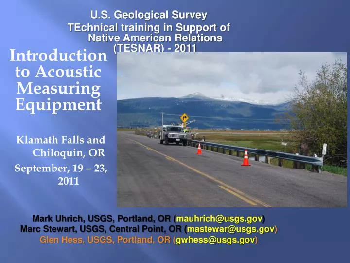
U.S. Geological Survey TEchnical training in Support of Native American Relations (TESNAR) - 2011. Introduction to Acoustic Measuring Equipment Klamath Falls and Chiloquin , OR September, 19 – 23, 2011. Mark Uhrich , USGS, Portland, OR ( mauhrich@usgs.gov )

E N D
U.S. Geological Survey TEchnical training in Support of Native American Relations (TESNAR) - 2011 Introduction to Acoustic Measuring Equipment Klamath Falls and Chiloquin, OR September, 19 – 23, 2011 Mark Uhrich, USGS, Portland, OR (mauhrich@usgs.gov) Marc Stewart, USGS, Central Point, OR (mastewar@usgs.gov) Glen Hess, USGS, Portland, OR (gwhess@usgs.gov)
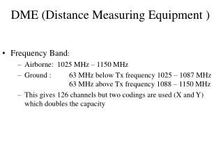
Brief History of ADCPS • Ocean going boats used “speed logs” to measure speed of the boat. • “The first commercial ADCP, produced in the mid-1970’s,was an adaptation of a commercial speed log” (Rowe and Young, 1979). • 1980s Doppler technology continue to involve • Early 1990s ADCP become more widespread in the USGS and other agencies. • 2012 Acoustic based instruments become the most common instrument type used in the USGS (Flowtrackers and ADCPs)
Acoustic Instrument What Why and When Much of the material in the presentation is borrowed from USGS Hydroacoustic Classes
Acoustic Instruments TRDI StreamPro TRDI Rio Grande ADCP SonTek RiverSurveyor SonTek Flow Tracker
FlowTracker (acoustic point measurements) • Ceramic transducers send and receive pulses of sound • Center transducer transmits the sound, while the transducers on the arms are receivers • Location of velocity measurement is called the sample volume • Sample volume is located about 4 inches from the transmitting transducer • Measures velocity based on the Doppler shift
What Is an ADCP?LET’S LOOK AT THE NAME“a” “d” “c” “p” Acoustic Sound Waves and the Doppler Doppler Shifts are used to measure Current Water Velocity Profiler Profiles
Sound Waves Trumpet ADCP Transducer Water wave crests and troughs are points of high and low water elevations. + Crest Trough - Sound wave “crests” and “troughs” consist of bands of high and low air or water pressure.
How does an ADCP instrument work? • Uses Doppler shift to measure water velocity • The Doppler effect is the change in a sound's observed pitch (frequency) caused by the relative velocities of the sound source and receiver.
The Basic Doppler Equation fD=fS *V/C fD= Doppler Shifted Frequency fS= Source Frequency (frequency of ADCP) V = Velocity of scatterers in water C = Speed of Sound (dependent on water char.)
Scatter Velocity Assumption V=fD / 2fS * C V = water velocity = scatterer velocity Important We assume that, on average, scatterer velocity equals water velocity Violation of this assumption will lead to errors in water velocity computation. Note: The 2 in the equation is result of two Doppler shifts, oneas the sound goes out and another as it returns
Fish: Water Water Water-velocity measurement is biased toward the fish velocity Stationary object: Rock Water-velocity measurement is biased toward zero When the scatter velocity may not be equal to the water velocity
Importance of Speed of sound (C) V=(fD /2fS *)C Important Speed of sound (C) must be computed accurately by the instrument. • A temperature error of 4o C or salinity error of 12 ppt will result in a 1% velocity error • The instrument must have an accurate temperature sensor and must be configured for the correct salinity • Rule of thumb: Specific conductance generally below 5000 uS/cm should not significantly affect C • Policy: All acoustic instruments must have independent temperature check (within 2 degrees C)
Picture at time T1 Picture at time T2 ADCP Speed Analogy S • To measure velocity, ADCPs listen to the returns at two separate times V=S/(T2-T1)
Phase Phase is the fraction of a wave cycle elapsed relative to a point – or when thought of as the wheel on the left, how much it has rotated Usually ADCPs use PHASE CHANGE to measure the speed, instead of measuring the change in frequency of the wave (how far the cars have travelled)
Phase Change – Like measuring how much the wheels on the cars have rotated Picture 2 Picture 1 • Because we don’t know the direction the cars are traveling, we must account for both positive and negative values (we measure a half rotation either direction) • Set the time between pictures (lag) to optimize the tire rotationfor the expected speed– Longer time (lag) = more precise measurement • Too long of time between picture (long lag) may cause the distance car travels to exceeds a half rotation and result in a measurement error called ambiguity error • Short time (lag) limits precision (increased random noise), but decreases possibility of an ambiguity error
What Does This Mean? Lag = Time between pulses in a ping Long lag = accurate measurements Long lag = low ambiguity velocity Exceed ambiguity velocity = ambiguity error Ambiguity error = inaccurate measurements Lag needs to be optimized based on maximum speed SonTek usually has short lags (no chance for ambiguity errors but noisy – pictures close together and wheel hasn’t turned much in lower velocites) TRDI – usually has longer lags that need to be adjusted for conditions (less noise, but chance for ambiguity errors if not adjusted correctly)
Correlation How well the two pictures can be alignedIf there is too long of a time between pictures, cars may be in different locations relative to each other, or the to pictures could contain totally different cars and the distance S may not be determined S
Transducers Produce sound waves (pulses) and then listen to returning sound waves ceramic element protected with a urethane coating ADCPs use the same transducer to both transmits and receive the pulses.
Need Multiple Transducer Since each Transducer only measures the velocity component parallelto the beam, multiple transducers are needed 4 beams can be resolved into: x, y, z and error velocities M9 only uses 4 beams at a time to compute a velocity RiverRay forms 4 beams from the single phased array transducer
Velocity Errors The difference betweenbeam pair vertical velocitiesis reported in software as Error or D Velocity ? Non-homogeneous (High error or D velocity) Homogeneous (Low error velocity)
Error Velocity Contour • Error velocities should be randomly distributed • areas of high area error velocities may occur when water is not flowing at similar magnitudes and direction in all beams (example: turbulence) • Error velocities may also be the result of an instrument measuring one beam velocity wrong Behind Bridge Pier
Types of Pulses • How the pulses are transmitted into the water and sampled can vary and be optimized for the conditions • This configuration is commonly called “water mode” • Some of the newer ADCPs automatically adjust the configurations for the environment on the fly • Until recently the majority of ADCPs currently in use must be set up prior to data collection
Depth Cells (Bins) Transmitting Blanking Gate 4 Gate 2 Gate 3 Time Gate 1 end start B C A echo echo echo echo Blank Bin 1 cell 1 Bin 2 cell 2 Bin 3 cell 3 Distance From ADCP Bin 4 cell 4
ADCP’s Profile (Ensemble) Depth Cell
ADCP Measured Water Velocity The faster the boat travels, the faster the velocity of the water relative to the ADCP.
Boat Speed (Bottom Tracking) • ADCP’s can also measure the speed of the instrument or boat by measuring the Doppler shift of a pulse off of the bottom • This is called bottom tracking and assumes that the streambed is stationary • Sediment transport on or near the streambed can affect the Doppler shift of the bottom-tracking pulses, which can result in the measured boat velocity being biased in the opposite direction of the sediment movement. This is referred to as a Moving Bed condition
Depths • Bottom Track pulses are also used to measure depth • Typically 4 beam depths are averaged • SonTek also can use a vertical beam dedicated to depth
Acoustic Profiler Discharge Measurement A single pass across the river is called a transect, a discharge measurement is usually comprised of multiple transects averaged together
Computation of Discharge • Measured Q = ∑(V x A) • V = Velocity perpendicular to boat path for the ensemble • A = Depth Cell Size x Width • Width = boat speed x time since last valid ensemble • Assumption made: the measured boat and water velocities are representative of the boat and water velocities since the last valid data. The longer it has been since the last valid data, the greater the error may be in this assumption • The above is equal to the cross product of the boat and water speed x depth cell size and the time since last ensemble, which is how software computes Q in a depth cell
Measured and Unmeasured Areas Depth Valid Ensembles(Profiles) Top (Estimated) Layer Middle (Measured) Layer Bottom (Estimated) Layer Edges (Estimated)
How To Estimate Top and Bottom Q? Free surface f1 • Q in the top and bottom unmeasured areas is estimated for each ensemble, based on the measured data • The typical method is to use a power fit of the measured data, but other options are available when this is not valid Measured Estimated f2 Power fit Distance from the bed (Z), feet f3 f4 f5 fn Velocity cross product (X-value), ft2/s2
Power Curve Limitations Bi-directional Flow Unidirectional Flow Distance from the bed (Z), feet Distance from the bed (Z), feet (+) 0 (+) (-) (-) 0 Velocity cross product (f-value), ft2/s2
Examples of profiles affected by Wind Range from Bottom Range from Bottom Water Velocity Water Velocity • Depending on direction, wind can either cause the profile to bend either way at the water surface • The magnitude of this may cause the standard power fit to be a poor choice for top extrapolation, in this case the software has options to only use data near thesurface for estimating the top Q
MEASURE the edge distance. Average multiple ensembles to get an accurate depth and velocity dm=last measured depth Vm = last measured velocity L Vm L = distance from last ensemble to edge of water dm Estimating Shore Discharges Measured by ADCP Measured by User The averaged measured velocity is multiplied by the averaged measured depth, the measured length, and finally by a coefficient to account for the shape of the edge (.35 for triangle and .91 for square)
Ideal Reach From: Water Resources Investigations Report 00-4036. By K. M. Nolan and Shields Online Training Class SW1271
Computation of Total Discharge Top Q Left Q Middle Q Right Q Bottom Q Total Q = Left Q + Right Q + Top Q + Bottom Q + Middle Q
Where ….Ideal Reach Reach - Straight and uniform for a distance that provides for uniform flow Streambed - stable free of large rocks, weeks or other obstructions A poor cross section = poor measurement regardless of the accuracy of your point velocities From: Water Resources Investigations Report 00-4036. By K. M. Nolan and Shields Online Training Class SW1271
Site Selection Still Critical • Reach - Straight and uniform for a distance that provides for uniform flow • Streambed - stable free of large rocks, weeks or other obstructions • A poor cross section = poor measurement regardless of the accuracy of your point velocities