Download
1 / 17
170 likes | 284 Vues
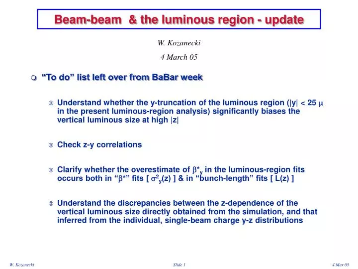
Beam-beam & the lum in ous region - update. W. Kozanecki 4 March 05. “To do” list left over from BaBar week Understand whether the y-truncation of the luminous region (|y| < 25 m in the present luminous-region analysis) significantly biases the vertical luminous size at high |z|

E N D
Beam-beam & the luminous region - update W. Kozanecki 4 March 05 • “To do” list left over from BaBar week • Understand whether the y-truncation of the luminous region (|y| < 25 m in the present luminous-region analysis) significantly biases the vertical luminous size at high |z| • Check z-y correlations • Clarify whether the overestimate of b*y in the luminous-region fits occurs both in “b*” fits [ s2y(z) ] & in “bunch-length” fits [ L(z) ] • Understand the discrepancies between the z-dependence of the vertical luminous size directly obtained from the simulation, and that inferred from the individual, single-beam charge y-z distributions
z ~ 0 z ~ 16 mm L/bunch (1024 cm-2 s-1) z ~ 26 mm Y (m) Any truncation bias at high |y|, high |z| ? Could the systematic discrepancy in syL at high z, be due to y-truncation imposed in the luminosity computation by the simulation?
So far ignored z-slice info in b-b sim output, i.e. assumed x, y, z uncorrelated Now ‘sample’ each z slice as it crosses the IP, i.e. plot y*, yp = f( zslice) (y*) low I e- bunch <-- tail head --> dN/dy* e+ z (mm) y-z correlations in single-beam charge distributions
Single-beam y-z correlations : low vs. high current (y*) low I e- (yp) low I bunch <-- tail head --> e+ (y*) high I • Y. Cai: “pinch effect” ! • akin to what is happening in LC • distinct from dyn. (yp) High I
z-dependence of effectivey, *y : high current *yeff , high current yeff , high current e+ e+ e- e-
z-dependence of effectivey, *y : low current *yeff , low current yeff , low current e+ e- e+ e- Could the “low current” still be too high? Ilya will generate a very low current data set
b*y ‘measurements’ (on b-b simulations, no detector effects!) • e, b* = simulation input parameters • Compute effective values of e, b* (LER or HER) from e+/e- charge distributions: sy = e b*y s’y = e / b*y • Fit z-dependence of vertical beam size (LER or HER): s2y (z) = sy2 + s’y2 z2 = (e b*y)+ (e / b*y)z2 • Fit z-dependence of luminous region • z-dependence of vertical luminous size syL (z, by*LER, by*HER) (bunch-length independent) • longitudinal luminosity distribution L(z, by*LER, by*HER, sz, LER, sz, HER)
Single-beam y, b*y fits (updated for actual z-dependence) LER sy2 (z) (High current) LER sy2 (z) (Low current) LER High I Low I HER sy2 (z) (High current) HER sy2 (z) (Low current) HER
These results updated for y-z correlations Single-beam b*y fits(high/lowx)
Ly2 ~ z2 (2 parameters), but we need 4: yLER, yHER , yLER , yHER Several possibilities, e.g.: Fix yLER, yHER , yHERFit yLER Fix yHER / yLER , yHERFit yLER, yLER Fitting the z-dependence of the vertical luminous size syL (z) (m) syL (z) (m) Low current Low current z (mm) z (mm)
b*y fits(high/lowx) using the vertical -beam or -luminous size
Fixed -normalization method Fitting code from B. Viaud Bunch length fits to L(z) distribution (high/lowx)
Fit z+ only Fit z+, y+ Why is the fitted bunch length so stable? L (arb. units) L(z) appears insensitive to * for |z| < 20 mm Fit z+ only Ratio of fitted functions Fit z+ only Fit z+, y+ Fitted / ‘mrsd’ Fit z+, y+ z (mm) z (mm)
Summary (I) • A beam-beam ‘pinch effect’ is apparent in the z-slice dependence of the vertical beam sizes, resulting in large variations in effective vertical emittance & -function along the bunch. • the effect is spectacular at nominal bunch current • it may still be significant at low (10%) bunch current, and may be responsible for the small bias observed in the single-beam *y fits. • The bunch length fit [ L(z) ] and the fit to the vertical luminous size [ yL(z) ] return b*y values consistent with each other, but overestimated by ~ 4-5 mm (as suggested by real data). This bias may be due to the above-mentioned pinch effect. • Additional beam-beam simulations at very low current (1% nominal) are in progress to verify this interpretation. • Bunch-length fits of the longitudinal luminosity distribution • return the correct (MC truth) bunch length within < 5%, at both low & high x, under all considered b*y scenarios: • both b*y’s fixed to true (input) values • one or both b*y’s floated in the fit The robustness of the bunch length fit is attributed to the fact that *y does not significantly affects the L(z) distribution until |z| > 20 mm.
However... • Still open / to be understood in the simulation • is the pinch effect really the culprit, i.e. will we get the correct * from the luminous-region analyses at very low current (1% nominal) ? • what is the physics of the pinch effect? • how is it different from the dynamic- effect? • Is it effectively a steady-state phenomenon? • on what time scale (# turns) does it stabilize? • what diagnostics can we run on the simulation to understand it better? • why does the ‘pinch effect’ (if it really is the culprit) induce similar * distortions at nominal and at low (10%) bunch current? • the error treatement is not correct in the (simulated) luminous-region analyses, in that it ignores the peculiar statistical-fluctuation mechanism: in the simulation, fluctuations are driven by the # of macroparticles in each bin, not by the luminosity as in the real world). Could the bias be worse than the present studies suggests? (The statistical treatement of the single-beam simulations IS correct, though.) • ...and in the data • why does floating y change the fitted z+ value? • why does the data fit @ fixed y look bad, while the same fit on the simulation looks decent (up to clarifying the stat. error issues above) ?