Download
1 / 1
10 likes | 169 Vues
EnKF Localization Techniques and Balance 1 Steven J. Greybush, 1 Eugenia Kalnay, 1 Takemasa Miyoshi, 1 Kayo Ide, and 1 Brian Hunt 1 University of Maryland, College Park, MD, U.S.A. Origin of Imbalances and Differing Localization Strengths. Localization

E N D
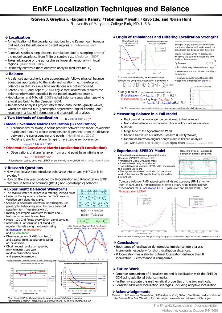
EnKF Localization Techniques and Balance 1Steven J. Greybush, 1Eugenia Kalnay, 1Takemasa Miyoshi, 1Kayo Ide, and 1Brian Hunt 1University of Maryland, College Park, MD, U.S.A. • Origin of Imbalances and Differing Localization Strengths • Localization • A modification of the covariance matrices in the Kalman gain formula that reduces the influence of distant regions. (Houtekamer and Mitchell, 2001) • Removes spurious long distance correlations due to sampling error of the model covariance from finite ensemble size. (Anderson, 2007) • Takes advantage of the atmosphere’s lower dimensionality in local regions. (Hunt et al., 2007) • Ultimately creates a more accurate analysis (reduces RMSE). Original (solid) and localized (dashed) Waveforms Imbalance of original and localized Waveforms Example adapted from Lorenc (2003). • Example: Apply a Gaussian localization function to a balanced h and v waveform based upon the distance from the origin. • |dh/dx| increases while |v| decreases, disrupting the balance between the wind field and the mass field. • By Analogy: • Assimilate height observation at origin. • Waveforms are proportional to analysis increments. • Example considers modification of K, irrespective of modification of B or R. L=250 km • Balance • A balanced atmospheric state approximately follows physical balance equations appropriate to the scale and location (i.e., geostrophic balance) so that spurious time oscillations are not introduced. • Lorenc (2003) and Kepert (2006) argue that localization reduces the balance information encoded in the model covariance matrix. • Houtekamer and Mitchell (2005) noted balance issues when applying a localized EnKF to the Canadian GCM. • Imbalanced analyses project information onto inertial-gravity waves, which are filtered out (geostrophic adjustment, digital filtering, etc.), resulting in a loss of information and a suboptimal analysis. • To understand the differing localization strength, • consider two grid points, observation at grid point 1. • K for grid point 2: (d12 = distance between grid points) • B localization K2 = fBloc(d12)B12 (B11 + R1)-1 • R localization K2 = B12 (B11+fRloc(d12)R1)-1 • = fBloc(d12)B12 (fBloc(d12)B11+ R1)-1 = Localization Distance L Localization function floc Note: This comparison is more complex in the case of simultaneous assimilation of multiple observations. • Measuring Balance in a Full Model • Two Methods of Localization • Model Covariance Matrix Localization (B Localization) • Accomplished by taking a Schur product between the model covariance matrix and a matrix whose elements are dependent upon the distance between the corresponding grid points. (Hamill et al., 2001) • Model grid points that are far apart have zero error covariance. • Observation Covariance Matrix Localization (R Localization) • Observations that are far away from a grid point have infinite error. K = BHT(HBHT + R)-1 • Background can no longer be considered to be balanced. • Natural imbalance vs. imbalance introduced by data assimilation Methods: • Magnitude of the Ageostrophic Wind • Second Derivative of Surface Pressure (Gravity Waves) • Difference between original analysis and initialized analysis (i.e., with Lynch and Huang (1992) digital filter) (Houtekamer and Mitchell, 2005) Bloc = B * exp(-(ri-rj)2 / 2L2) • Experiment: SPEEDY Model Observing System: Rawinsonde distribution at model grid points. • Simplified Parametrizations, primitivE-Equation DYnamics (SPEEDY) (Molteni, 2003) • Atmospheric Global Circulation Model • 7 vertical levels using σ-coordinates • horizontal spectral resolution of T30, which corresponds to a standard 96x48 grid • Five dynamical variables: zonal wind (u), meridional wind (v), temperature (T), specific humidity (q), surface pressure (ps) Rloc = R * exp(+(d)2 / 2L2) R localization can be used with LETKF where there is no explicit B. (Hunt 2005, Miyoshi 2005) • Research Questions • How does localization introduce imbalance into an analysis? Can it be avoided? • How do the analyses produced by B-localization and R-localization EnKF compare in terms of accuracy (RMSE) and (geostrophic) balance? Compare balance (RMS ageostrophic wind) and accuracy (RMS error from truth) in N.H. and S.H midlatitudes at level 4 (~500 hPa) in identical twin experiments for B-Localization EnSRF (Whitaker and Hamill, 2002), and R-Localization LETKF. • Experiment: Balanced Waveforms • The shallow water equations in a rotating, inviscid fluid: • Linearize the equations, solve for harmonic solution. Variation only along the x-axis. • Solution is sinusoidal waveform for h (height). Use geostrophic balance equation to create balanced waveform for v(meridional wind). • Initially geostrophic waveform for truth and 5 background ensemble members. • Model: 101 Grid Points every 50 km along domain. • Assimilate 40 observations of h and v at regular intervals along the domain using B localization, R localization, and no localization. • Observe accuracy (RMSE from truth) and balance (RMS ageostrophic wind) of the analysis. • Obtain robust results by repeating each scenario 100x with random observation errors and ensemble members. Initial Ensemble (dashed), Truth (solid), and Observations for height and meridional wind. Results reported as average over 30 days following 20 day spinup. Experiment took place in months of Feburary and March. • Conclusions • Both types of localization do introduce imbalance into analysis increments, especially for short localization distances. • R localization has a shorter optimal localization distance than B localization. Performance is comparable. Distance between Observations D = 500 km; Wavelength W = 2000 km • Future Work • Continue comparison of B localization and R localization with the SPEEDY GCM using additional balance metrics. • Further investigate the mathematical properties of the two methods. • Consider additional localization strategies, including adaptive localization. • Acknowledgements • Thanks to UMD Weather Chaos Group, Jeff Anderson, Craig Bishop, Dale Barker, and attendees of the Buenos Aires D.A. Workshop for their helpful comments and critiques of this project. Note: Use LETKF for R-localization to avoid undesired statistical properties (asymmetric B-matrix). Results are very similar to EnSRF, so the comparison is fair. The 5th WMO Symposium on Data AssimilationMelbourne, Australia; October 5-9, 2009