Download
1 / 53

E N D
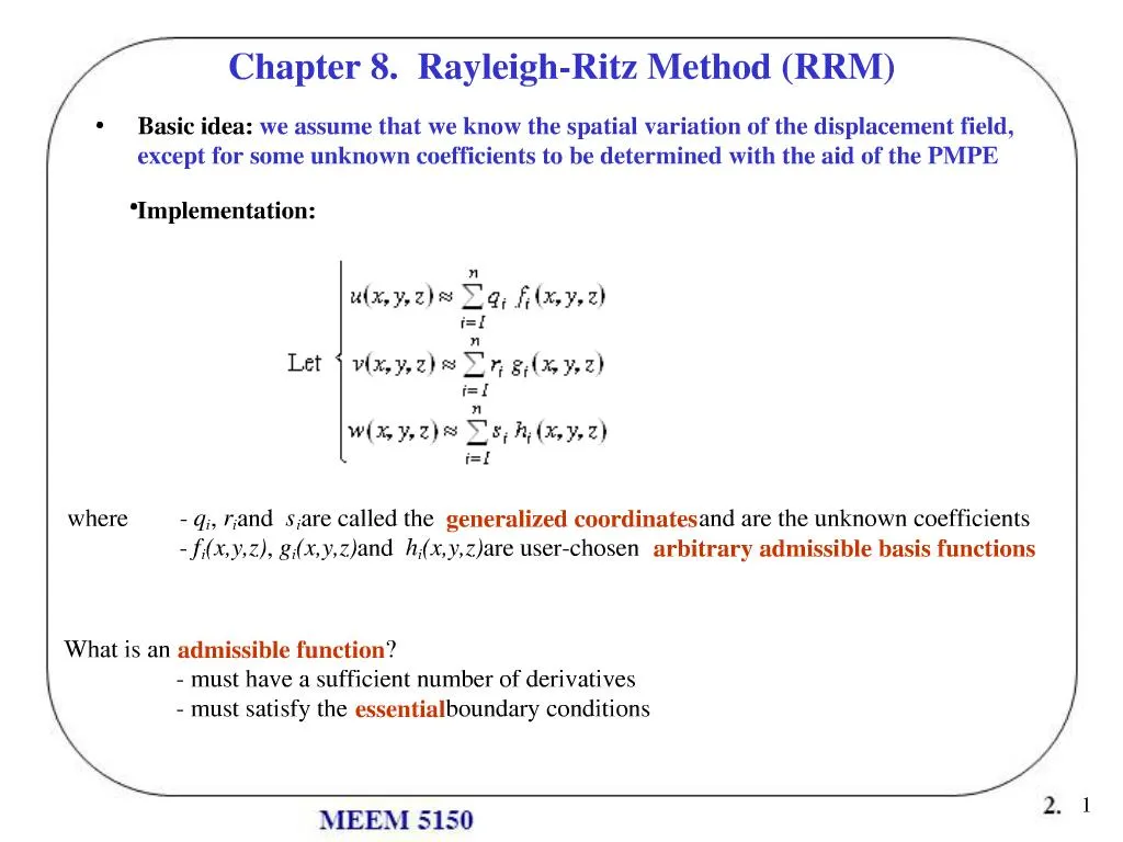
1. 1 Chapter 8. Rayleigh-Ritz Method (RRM) Basic idea: we assume that we know the spatial variation of the displacement field, except for some unknown coefficients to be determined with the aid of the PMPE
2. 2 Rayleigh-Ritz Method Parenthesis : what is an essential boundary condition?
3. 3 Rayleigh-Ritz Method
4. 4 Rayleigh-Ritz Method Substitute the approximate displacement field into the total potential energy to get
Then apply the PMPE (or PVW)
Thus we end up with 3n equations for the 3n unknown coefficients (qi,ri,si).
This is an approximate method since (unless you are very lucky), the basis functions are not correct, thus u, v and w will be approximate. The closer the basis functions are to the exact spatial variation of the displacements, the better the approximation.
5. 5 RRM: applications
6. 6 Application 1 - Exact Solution
7. 7 Application 1 - First attempt
8. 8 Application 1 - Second attempt
9. 9 Application 2 - First attempt
10. 10 Application 2 - Second attempt
11. 11 RRM: final notes Conclusions
Advantages
Simplicity
�keep old terms� when adding new ones
Disadvantages
Basis functions are hard to find for complicated geometries (especially in 2-D and 3-D cases)
qi have no physical significance
Convergence is hard to quantify
12. 12 3. Basic concepts of FEM: solution of 1-D bar problem Table of contents
3.1 Basic concepts : mesh, nodes, elements, interpolation, ...
3.2 FEA of axially loaded bar
3.3 Notes : direct method, higher-order elements, �
3.4 Principle of Virtual Work (PVW) approach
3.5 Galerkin Weighted Residual (GWR) method
13. 13 3.1 Basic concepts The FEM is also based on the RRM, but
the basis functions are easy to find : interpolation
the qi have a physical significance : nodal displacements
Basic idea
Discretize the domain with a finite element mesh composed of nodes and elements
Compute the �best values� of the nodal displacements (based, for example, on the PMPE)
Use interpolation to find the solution everywhere else in the discretized domain
There are many elements of different types and geometries : 1-D, 2-D, 3-D, plane stress, plane strain, plates, shells, structural, thermal, fluid mechanics, electromagnetic, elastic, plastic, static, dynamic, �
14. 14 3.2 FEA of axially loaded bar In this section, we introduce the 6 basic steps of a FEA by solving the following simple structural problem
15. 15 FEA of axially loaded bar Finite element solution
We will use the PMPE. The total potential energy P for this problem is
16. 16 FEA of axially loaded bar
17. 17 Na(s) and Nb(s) play an important role in FEA and are called interpolation or shape functions FEA of axially loaded bar
18. 18 FEA of axially loaded bar Expand the square term :
19. 19 Since we know that
20. 20 FEA of axially loaded bar
21. 21 FEA of axially loaded bar Note : the approximate displacement solution is continuous within and between elements
Within an element :why?
Between elements : why?
22. 22 FEA of axially loaded bar Let�s add the contribution of all three elements to the total potential energy
23. 23 FEA of axially loaded bar
24. 24
25. 25 FEA of axially loaded bar
26. 26 FEA of axially loaded bar
27. 27 FEA of axially loaded bar
28. 28 FEA of axially loaded bar
29. 29 FEA of axially loaded bar
30. 30 FEA of axially loaded bar
31. 31
32. 32 FEA of axially loaded bar
33. 33 FEA of axially loaded bar
34. 34 3.3 Notes
35. 35
36. 36
37. 37 Notes (Cont�d)
38. 38 Notes (Cont�d)
39. 39 Notes (Cont�d)
40. 40 Notes (Cont�d)
41. 41 Two applications
42. 42 Notes (Cont�d)
43. 43 3.4 PVW approach
44. 44
45. 45 3.5 Galerkin Weighted Residual approach
46. 46
47. 47
48. 48 WRM: application
49. 49 WRM: application
50. 50 WRM: application
51. 51
52. 52
53. 53