Download
1 / 16
160 likes | 375 Vues
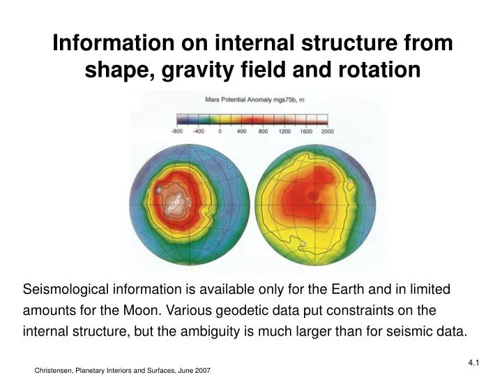
Information on internal structure from shape, gravity field and rotation. Seismological information is available only for the Earth and in limited amounts for the Moon. Various geodetic data put constraints on the internal structure, but the ambiguity is much larger than for seismic data.

E N D
Information on internal structure from shape, gravity field and rotation Seismological information is available only for the Earth and in limited amounts for the Moon. Various geodetic data put constraints on the internal structure, but the ambiguity is much larger than for seismic data.
Gravity field: fundamentals Gravitational potential V, Gravity (acceleration) g = - grad V Point mass: V = - GM/r (also for spherically symmetric body) Ellipsoid: General: General description of gravity field in terms of spherical harmonic functions. Degree ℓ=0 is the monopole term, ℓ=2 the quadrupole, ℓ=3 the octupole, etc. A dipole term does not exist when the coordinated system is fixed to the centre of mass. J, C, S are non-dimensional numbers. Note: J2 = -C2o (times a constant depending on the normalization of the Pℓm) Symbols [bold symbols stand for vectors]: G – gravitational constant, M –total mass of a body, r – radial distance from centre of mass, a – reference radius of planet, e.g. mean equatorial radius, θ – colatitude, φ – longitude, Pn – Legendre polynomial of degree n, Pℓm – associated Legendre function of degree ℓ and order m, Jn, Cℓm, Sℓm – expansion coefficients
Measuring the gravity field • Without a visiting spacecraft, the monopole gravity term (the mass M) can be determined by the orbital perturbations on other planetary bodies or from the orbital parameters of moons (if they exist) • From a spacecraft flyby, M can be determined with great accuracy. J2 and possibly other low-degree gravity coefficient are obtained with less accuracy • With an orbiting spacecraft, the gravity field can be determined up to high degree (Mars up to ℓ ≈ 60, Earth up to ℓ ≈ 180) • The acceleration of a spacecraft orbiting (or passing) another planet is determined with high accuracy by radio-doppler-tracking: The Doppler shift of the carrier frequency used for telecommunication is proportional to the line-of-sight velocity of the spacecraft relative to the receiving antenna. Δv can be measured to much better than a mm/sec. • On Earth, direct measurements of g at many locations complement other techniques. • The ocean surface on Earth is nearly an equipotential surface of the gravity potential. Its precise determination by laser altimetry from an orbiting S/C reveals small-wavelength structures in the gravity field.
ρ ρuncompressed Mantle Outer Inner core Mean density and uncompressed density From the shape (volume) and mass of a planet, the mean density ρmean is obtain-ed. It depends on chemical composition, but through self-compression also on the size of the planet (and its internal temperature; in case of terrestrial planets only weakly so). In order to compare planets of different size in terms of possible differ-ences in composition, an uncompressed density can be calculated: the mean density it would have, when at its material where at 1 bar. This requires knowledge of incompressibility k (from high-pressure experiments or from seismology in case of the Earth) and is approximate. ρmeanρuncompressed Earth 5515 4060 kg m-3 Moon 3341 3315 kg m-3 The mean density alone gives no clue on the radial distribution of density: a body could be an undifferentiated mixture (e.g. of metal and silicate, or of ice and rock in the outer solar system), or could have separated in different layers (e.g. mantle and core).
Moment of inertia L = IωL: Angular momentum, ω: angular frequency, Imoment of inertia for rotation around an arbitrary axis, s is distance from that axis I is a symmetric tensor. It has 3 principal axes and 3 principal components (maximum, intermediate, minimum moment of inertia: C ≥ B ≥ A.) For a spherically symmetric body rotating around polar axis compare with integral for mass In planetary science, the maximum moment of a nearly radially symmetric body is usually expressed as C/(Ma2), a dimensionless number. Its value provides information on how strongly the mass is concentrated towards the centre. C/(Ma2)=0.4 2/3 →0 0.347 for ac=a/2, ρc=2ρm 0.241 for ac=a/2, ρc=10ρm Homogeneous sphere Hollow shell Small dense core thin envelope Core and mantle, each with constant density Symbols: L – angular momentum, I moment of inertia (C,B,A – principal components), ω rotation frequency, s – distance from rotation axis, dV – volume element, M – total mass, a – planetary radius (reference value), ac – core radius, ρm – mantle density, ρc –core density
Determining planetary moments of inertia McCullagh‘s formula for ellipsoid (B=A): In order to obtain C/(Ma2), the dynamical ellipticity is needed: H = (C-A)/C. It can be uniquely determined from observation of the precession of the planetary rotation axis due to the solar torque (plus lunar torque in case of Earth) on the equatorial bulge. For solar torque alone, the precession frequency relates to H by: When the body is in a locked rotational state (Moon), H can be deduced from nutation. For the Earth TP = 2π/ωP = 25,800 yr (but here also the lunar torque must be accounted) H = 1/306 and J2=1.08×10⁻³ C/(Ma2) = J2/H = 0.3308. This value is used, together with free oscillation data, to constrain the radial density distribution. Symbols: J2 – gravity moment, ωP precession frequency, ωorbit – orbital frequency (motion around sun), ωspin – spin frequency, ε - obliquity
Centrifugal force Extra gravity from mass in bulge Determining planetary moments of inertia II For many bodies no precession data are available. If the body rotates sufficiently rapidly and if its shape can assumed to be in hydrostatic equilibrium [i.e. equipotential surfaces are also surfaces of constant density], it is possible to derive C/(Ma2) from the degree of ellipsoidal flattening or the effect of this flattening on the gravity field (its J2-term). At the same spin rate, a body will flatten less when its mass is concentrated towards the centre. Darwin-Radau theory for an slightly flattened ellipsoid in hydrostatic equilibrium measures rotational effects (ratio of centrifugal to gravity force at equator). Flattening is f = (a-c)/a. The following relations hold approximately: Symbols: a –equator radius, c- polar radius, f – flattening, m – centrifugal factor (non-dimensional number)
Structural models for terrestrial planets Assuming that the terrestrial planets are made up of the same basic components as Earth (silicates / iron alloy with zero-pressure densities of 3300 kg m-3 and 7000 kg m-3, respectively), core sizes can be derived. Ambiguities remain, even when ρmean and C/Ma2 are known: the three density models for Mars satisfy both data, but have different core radii and densities with different sulphur contents in the core.
Interior of Galilean satellites From close Galileo flybys mean density and J2 (assume hydrostatic shape C/(Ma2)) Low density of outer satellites substantial ice (H2O) component. Three-layer models (ice, rock, iron) except for Io. Assume rock/Fe ratio. Callisto‘s C/Ma2 too large for complete differentiation core is probably an undifferen-tiated rock-ice mixture.
1000 km HST images Ceres From HST images, the flattening of Ceres has been determined within 10%. Its mean density, 2080 kg m-3, hints at an ice-rock mixture. The flattening is too small for an undifferentiated body in equilibrium. From Darwin-Radau theory, C/Ma2≈ 0.34. Models with an ice mantle of ~120 km thickness above a rocky core agree with the observed shape. [Recent result that needs confirmation]
Δh Airy model ρc ρm>ρc Gravity anomalies Gravity anomaly Δg: Deviation of gravity (at a reference surface) from theoretical gravity of a rotating ellipsoidal body. Geoid anomaly ΔN: Deviation of an equipotential surface from a reference ellipsoid (is zero for a body in perfect hydrostatic equilibrium). Isostasy means that the extra mass of topographic elevations is compensated, at not too great depth, by a mass deficit (and vice versa for depressions). In the Airy model, a crust with constant density ρcis assumed, floating like an iceberg on the mantle with higher density ρm. A mountain chain has a deep crustal root. When the horizontal scale of the topography is much larger than the vertical scales, the gravity anomaly for isostatically compensated topography is approximately zero. Without compensation, or for imperfect compensation, a gravity anomaly is observed. Also for very deep compensation (depth not negligible compared to horizontal scale) a gravity anomaly is found.
Δg Δg Δg Low density crust Strong thick lithosphere Δg Deep low-density body Δh ↨ lithosphere Thin elastic Examples for different tectonic settings No compensation Shallow compensation Deep compensation Elastic flexure
Mars gravity field Comparing the gravity anomaly of Mars with the topographic height, we can conclude: Tharsis volcanoes not compensated, only slight indication for elastic plate bending volcanoe imposed surficially on thick lithosphere Hellas basin shows small gravity anomaly compensated by thinned crust Valles Marineris not compensated Topographic dichotomy (Southern highland, Northern lowlands) compen-sated crustal thickness variation Tharsis bulge shows large-scale positive anomaly. Because incomplete compensation is unlikely for such broad area, deep compensation is must be assumed (for example by a huge mantle plume) Δg Valles Marineris Tharsis Δh Hellas
Sun Forced librations of Mercury View on the North pole Mercury‘s rotation is in a 3:2 resonance with its orbital motion. For each two revolutions around the sun, it spins 3 times around its axis. This state is stabilized (against slowing down by tidal friction) by the strong eccentricity e=0.206 of Mercury‘s orbit. The orbital angular velocity follows Kepler‘s 2nd law and while being on average 2/3 of the spin rate, it exceeds the spin rate slightly at perihelion, where the sun‘s apparent motion at a fixed point on Mercury‘s surface is retrograde. At perihelion tidal effects are largest and here they accelerate the spin, rather than slowing it down like in other parts of the orbit. Mercury is slightly elongated in the direction pointing towards the sun when it is at perihelion. The solar torque acting on the excess mass makes the spin slightly uneven. This is called a forced (or physical) libration. Δg Δh Hellas
Mantle Fluid core Solid core Forced librations of Mercury The libration angle Φ indicates the deviation of the orientation of a fixed point on the planet from that expected for uniform rotation. Φ varies periodically over a Mercury year. Its amplitude Φo depends on whether the whole planet follows the libration, or if the mantle can slip over fluid layer in the outer core. In the latter case, the libration amplitude is larger. The libration amplitude is proportinal to Cm/(B-A), where Cm indicates the moment of inertia of the mantle; more precisely: of that part of the planet that follows the librational motion. Δg Cm/C=1 would indicate a completely solid core, Cm/C < 1 a (partly) liquid core. (B-A)/(Ma2) = 4C22. From Mariner 10 flybys C22≈ (1.0±0.5) x 10-5 C/Ma2 can be estimated to be in the range 0.33 – 0.38. Φo = 36 ± 2 arcsec has recently been measured using radio interferometry with radar echos of signals from ground-based stations. Δh Hellas
Margot et al., Science, 2007 Forced librations of Mercury • The accuracy of the derived value of Cm/C is strongly affected by the large uncertainty on the C22 gravity term (50% error). But the probability distribution for Cm/C is peaked around a value of 0.5. The probability for values near one is small. • It is likely that Mercury has a (partly) liquid core, • This agrees with the observation of an internal magnetic field. The operation of a dynamo (the most likely cause for Mercury‘s field) requires a liquid electrical conductor. Δg Δh Hellas