Download
1 / 19
210 likes | 360 Vues
Central Tendency. Mechanics. Notation. When we describe a set of data corresponding to the values of some variable, we will refer to that set using an uppercase letter such as X or Y.

E N D
Central Tendency Mechanics
Notation • When we describe a set of data corresponding to the values of some variable, we will refer to that set using an uppercase letter such as X or Y. • When we want to talk about specific data points within that set, we specify those points by adding a subscript to the uppercase letter like X1 • X = variable Xi = specific value
Example 5, 8, 12, 3, 6, 8, 7 X1, X2, X3, X4, X5, X6, X7
Summation • The Greek letter sigma, which looks like , means “add up” or “sum” whatever follows it. • For example, Xi, means “add up all the Xis”. • If we use the Xis from the previous example, Xi = 49 (or just X).
Example X= 82 + 66 + 70 + 81 + 61 = 360 Y= 84 + 51 + 72 + 56 + 73 = 336 (X-Y)= (82-84) + (66-51) + (70-72) + (81-56) + (61-73) = -2 + 15 + (-2) + 25 + (-12) = 24 X2= 822 + 662 + 702 + 812 + 612 = 6724 + 4356 + 4900 + 6561 + 3721 = 26262 One can also see it as (X2) (X)2= 3602 = 129600
Calculations of Measures of Central Tendency • Mode = Most commonly occurring value • May have bimodal, trimodal etc. distributions. • A uniform distribution is one in which every value has an equal chance of occurring • Median • The position of the median value can then be calculated using the following formula:
Median • If there are an odd number of data points: (1, 2, 2, 3, 3, 4, 4, 5, 6) • The median is the item in the fifth position of the ordered data set, therefore the median is 3.
Median • If there are an even number of data points: (1, 2, 2, 3, 3, 4, 4, 5, 6, 793) • The formula would tell us to look in the 5.5th place, which we can’t really do. • However we can take the average of the 5th and 6th values to give us the median. • In the above scenario 3 is in the fifth place and 4 is in the sixth place so we can use 3.5 as our median.
The Arithmetic Mean • For example, given the data set that we used to calculate the median (odd number example), the corresponding mean would be: • Note that they are not exactly the same. • When would they be?
Example: Slices of Pizza Eaten Last Week Value Freq Value Freq 0 4 8 5 1 2 10 2 2 8 15 1 3 6 16 1 4 6 20 1 5 6 40 1 6 5 • This raises the issue of which measure is best
Other Means • Geometric mean • Harmonic mean • Compare both to the Arithmetic mean of 3.8
Other Means • Weighted mean • Multiply each score by the weight, sum those then divide by the sum of the weights.
Trimmed mean • You are very familiar with this in terms of the median, in which essentially all but the middle value is trimmed (i.e. a 50% trimmed mean) • But now we want to retain as much of the data for best performance but enough to ensure resistance to outliers • How much to trim? • About 20%, and that means from both sides • Example: 15 values. .2 * 15 = 3, remove 3 largest and 3 smallest
Winsorized Mean 1 2 2 2 3 3 3 3 3 3 4 4 4 4 4 5 5 6 8 10 3 3 3 3 3 3 3 3 3 3 4 4 4 4 4 5 5 5 5 5 • Make some percentage of the most extreme values the same as the previous, non-extreme value • Think of the 20% Winsorized mean as affecting the same number of values as the trimming • Median = 3.5 • Huber’s M1 = 3.56 • M.20 = 3.533 • WM.20 = 3.75 • Mean = 3.95 • Which of these best represents the sample’s central tendency?
M-estimators • Wilcox’s text example with more detail, to show the ‘gist’ of the calculation1 • Data = 3,4,8,16,24,53 • We will start by using a measure of outlierness as follows • What it means: • M = median • MAD = median absolute deviation • Order deviations from the median, pick the median of those outliers • .6745 = dividing by this allows this measure of variance to equal the population standard deviation • When we do will call it MADN in the upcoming formula • So basically it’s the old ‘Z score > x’ approach just made resistant to outliers
M-estimators • Median = 12 • Median absolute deviation • -9 -8 -4 4 12 41 4 4 8 9 12 41 • MAD is 8.5, 8.5/.6745 = 12.6 • So if the absolute deviation from the median divided by 12.6 is greater than 1.28, we will call it an outlier • In this case the value of 53 is an outlier • (53-12)/12.6 = 3.25 • If one used the poorer method of using a simple z-score > 2 (or whatever) based on means and standard deviations, it’s influence is such that the z-score of 1.85 would not signify it as an outlier
M-estimators • L = number of outliers less than the median • For our data none qualify • U = number of outliers greater than the median • For our data 1 value is an upper outlier • B = sum of values that are not outliers • Notice that if there are no outliers, this would default to the mean
M-estimators • Compare with the mean of 181