Download
1 / 83
860 likes | 1.08k Vues
Cognitive Psychology. Attention. Overview. Exam Detection. Filtering and selection. Search. Automatic processing. Concentration. Maybe If We’re Lucky: Spotlight Inhibition of Return PRP Change Blindness Simon Effect Attention in sports. What do these have in common?.

E N D
Cognitive Psychology Attention
Overview Exam Detection. Filtering and selection. Search. Automatic processing. Concentration Maybe If We’re Lucky: Spotlight Inhibition of Return PRP Change Blindness Simon Effect Attention in sports
What do these have in common? You are driving to a lunch date, and accidentally take the route to your job. After you correct your route, as you are driving by the theatre, a red ball chased by a child suddenly appears on the street, and you screech your brakes. You get to the restaurant and try to find your friend, who has flaming red hair. The restaurant is packed, it’s hard to make-out faces, but you can see people’s hair so you look for red hair. When you get to your table your friend asks if you noticed the Star Wars promotion with two costumed people fighting with light sabers. As you talk about important but dull business, your mind keeps drifting to your exciting first date last night. You force yourself not to think about it, but it keeps coming back.
Innatentional Blindness (UK cycling commercial) • http://www.youtube.com/watch?v=Ahg6qcgoay4&eurl=http://www.dothetest.co.uk/ • Attentional Resources (Tide commercial) • http://www.youtube.com/watch?v=vgtfC5LBAW4
What do these have in common? • Detection. • Filtering and selection. • Search. • Automatic processing. • Concentration. The common element is attention.
Architecture The box model: Sensory Store Filter Pattern Recognition Selection STM LTM Input (Environment) Response
Attention • In this model, attention is: • The filter and selection boxes • The arrows. • The special job carried out by each of these boxes according to different theories of attention • (Yes, this is cheating) • In this model attention: • Puts together information from various sources. • Gets information into STM • Works in imagery
Attention • Highlights parts of the environment and blocks other parts. • Primes a person for speedy reaction. • Helps you retain information.
Attention • As you can see from the attempts to define it, attention is usually defined as what it does. As a result, we’re going to study it as five kinds of things. • Detection. • Filtering and selection. • Search. • Automatic processing. • Concentration.
Quizz We discussed five aspects of attention. Which of the following was not one: • selection c. forgetting b. automaticity d. concentration
Themes • Early or Late?In other words, when does “meaning” stamp the stimulus • What is it? • Some sort of bottleneck or filter? • A capacity or resource (or several kinds)? • Can we learn something by looking for it in brains?
Detection • Two kinds of thresholds: • Absolute Threshold: Minimum amount of stimulation required for detection. • Difference Threshold (“Just Noticeable Difference”): Amount of change necessary for two stimuli to be perceived as different.
Detection • Absolute Thresholds: • Vision: One candle, on a mountain, perfectly dark, 30 miles. • Hearing: A watch ticking 20 feet away. • Smell: A single drop of perfume in a three room apartment. • Touch: The wing of a bee on your cheek. • Taste: One teaspoon of sugar in two gallons of water.
Determining Thresholds • How to determine thresholds: • Method of limits: • Ascending: Start with a value below the threshold, increase, ask for detection, increase… At the point a person says “detect,” average that stimulus value with the value from the previous trial. Repeat to estimate threshold. • Descending: Same, but start above threshold and work down. • Combining results from both directions will give you an estimate of the threshold.
Determining Thresholds • How to determine thresholds: • Method of constant stimuli: • Present a series of randomly selected stimulus values, ask for yes/no response for each. The value that’s detected 50% of the time is the threshold. • These methods can be adapted to determine difference thresholds.
Determining Thresholds • We think thresholds work like a step function, but they don’t. They are sigmoid or ogive curves This graph represents an ‘ogive-curve’ and how detection really changes – it is a gradual slope. The threshold is defined as a 50% detection rate. This graph represents a step function. Below the threshold there is 0% detection. Above the threshold, there is 100% detection. This is the way we normally believe our perception to work.
Quizz Methods introduced by Fechner included • method of constant stimuli • method of limits, ascending • method of limits, descending • method of constant sorrow
Determining Thresholds • Difference Threshold: • Weber’s Law: K = ΔI / I • K is the Konstant • Δ is the difference • I is the stimulus intensity • The formula states that the threshold for noticing a difference (whether it’s the length of a line or weight of a dumbell) is a constant ration between the ‘old’ / background stimulus and the ‘new’ / target stimulus.
Determining Thresholds • But there is a problem: Thresholds Shift These are ogive curves for stimuli of the same intensity but with different signal to noise ratios or payoff matrix • How to get around this problem: A model that accounts for signal to noise ratios and payoff matrixes Signal Detection Theory
Weber’s Law states that • The just noticeable difference is a constant ratio of the original stimulus. • attention is a process of selecting and ignoring. • what goes up must come down. • the noise distribution is false
Signal Detection • Can estimate detection (sensitivity) independent of bias. • Two kinds of trials: • Noise alone: Background noise only. • Signal+noise: Background noise with signal. • Two responses from observer: • Detect. • Don’t detect.
Hits(response “yes” on signal trial) Criterion N S+N Probability density Say “no” Say “yes” Internal response
Correct rejects(response “no” on no-signal trial) Criterion N S+N Probability density Say “no” Say “yes” Internal response
Misses(response “no” on signal trial) Criterion N S+N Probability density Say “no” Say “yes” Internal response
False Alarms(response “yes” on no-signal trial) Criterion N S+N Probability density Say “no” Say “yes” Internal response
Signal Detection:Sensitivity and Bias • We can estimate two parameters from performance in this task: • Sensitivity: Ability to detect. • Good sensitivity = High hit rate + low false alarm rate. • Poor sensitivity = About the same hit and false alarm rates. • Response Bias: Willingness to say you detect. • Can be liberal (too willing) or conservative (not willing enough). • For example, if the true signal to noise ratio is 50% and you have a 75% detection rate, then your response bias is to be too liberal.
Signal Detection:Sensitivity and Bias • Computing sensitivity or d’ (“d-prime”) • Is a measure of performance (like percent correct, or response time) • Typical values are from 0 to 4 (greater than 4 is hard to measure because performance is so close to perfect) • A d-prime value of 1.0 is often defined as threshold.
d’ N S+N Probability density Internal response d-Prime • d-prime is the distance between the N and S+N distributions • d-prime is measure in standard deviations (Z-Scores) • In SDT, one usually assumes the two underlying distributions are normal with equal variance (i.e., both curves have the same standard deviation)
Signal Detection:Sensitivity and Bias • Computing bias: • The criterion is the point above which a person says “detect.” It can be unbiased (the point where the distributions cross; 1.0), liberally biased (< 1.0), or conservatively biased (> 1.0).
Signal Detection:Sensitivity and Bias • Since sensitivity and bias are independent, you can measure the effect of different biases on responding to a particular value for detectability. • Influences on bias: • Instructions (only say “yes” if you’re absolutely sure). • Payoffs (big reward for hits, no penalty for false alarms). • Probability of signal (higher probability leads to more liberal bias).
Signal Detection:Sensitivity and Bias • Receiver operating characteristic (ROC) curves: • For a given detectability value, you can manipulate the hit and false alarm rates. An ROC curve shows the effect of changing bias for that level of detectability.
Very sensitive observer Moderately sensitive observer Zero sensitivity Sample ROC Curves % of Hits
Optimal Performance • Depending on the probability of a signal trial and the payoff matrix, the optimal placement of the criterion will vary. p(N) value (CR) - cost (FA) opt = X p(S) value (H) - cost (M) • You can compare performance to the ideal observer to assess the operator.
Quizz • The Titanic hitting an iceberg would be a pretty good example of a • hit • miss • false alarm • correct rejection
Quizz Bob, an electrician, is trying to see how faint he can make a light. He starts by turning the light ON to its maximum, then turning it down until he cannot see it. a) Difference detection; methods of limits; ascending b) Difference detection; method of constant stimuli; random c) Absolute thresholds; method of limits; descending d) Absolute thresholds; constant stimuli; random
Quizz In Signal Detection Theory, which of the following is not true: • attention requires more hits than false alarms • there is a normal distribution for signal and one for noise with the distance apart measured in Z-scores • d-prime measures the difference between signal and noise • bias and sensitivity are independent
Filtering • How do we choose what to attend to? Is the choice made early or late? • We’ll look at several versions of filter models and some of the evidence.
Filter Pattern Recognition Sensory Store Selection Short-term memory Attended Unattended Filtering • Early: Broadbent. Selection happens at the filter and sensory store before pattern recognition. The selection is made at the EARLY STAGE of crude physical analysis.
“7-4-1” “3-2-5” Filtering • Early: Evidence: • Dichotic listening. Two messages, one to each ear, played simultaneously. • Shadowing: Repeat out loud everything in one ear. What do people (or what don’t people) notice in the unattended ear? • Miss change of speaker. • Miss change of language. • Miss change of direction.
Filtering • Early: Evidence: • Filter flapping: Two sets of numbers come in, one set in each ear. • Report by ear: Easy. • Report in order: Hard. • The argument is that the filter lets in all of one channel, then the other, no problem. To switch back and forth takes a lot of effort. “7-4-1” “3-2-5”
Filtering • Problem for early models: • People detect their name on the unattended channel (cocktail party phenomenon). • Treisman (1960): If a shadowed story switches ears, people follow it, and then correct. They have to be attending to meaning to follow the story.
Filtering • Problem for early models: • Example 1: • …I SAW THE GIRL/song was WISHING… • …me that bird/JUMPING in the street… • Example 2: • …AT A MAHOGANY/three POSSIBILITIES… • …look at these/TABLE with her head…
Pattern Recognition Sensory Store Selection Short-term memory Filter Attended Unattended Filtering • Attenuation model: • Everything in memory is active at some resting level. Some stuff that’s important has a high resting level, making it easier to respond to (e.g., your name). • Other stuff has a lower resting level, making it harder to respond to. • As you think about something, you raise its resting level.
Filtering • Attenuation model: • The unshadowed ear is attenuated (the volume is low). This little bit of attention can reach something with a high resting level (your name, a story you’re shadowing), but not some random bit of information. • So, no filter, just attenuation.
Filtering • Capacity model: • You have a certain amount of attention, you can spread it around as needed. If you spend a lot on one task, then you have less for others. • Primary task: Do well on this no matter what (main focus of resources). • Secondary task: Also do this. • By manipulating the difficulty of the primary task and measuring the secondary task, we can see how attention allocation affects performance.
Filtering • Capacity model: • For example, Johnston and Heinz (1978) had two tasks: • Primary: Shadow one ear. This can be based on gender or category. • Secondary: Detect a light.
Filtering • Capacity model: • What this implies is that the filter can be early (gender) or late (category), the amount of your resources that you allocate to it determines where the filter is.