Download
1 / 54
540 likes | 704 Vues
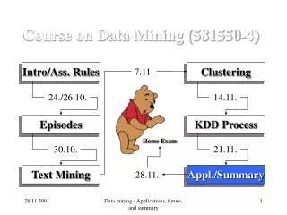
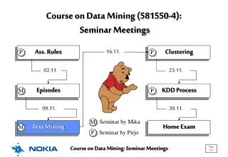
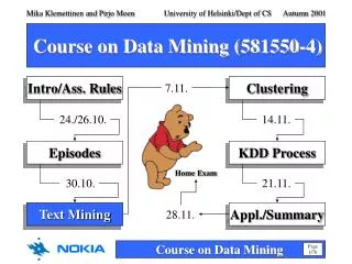
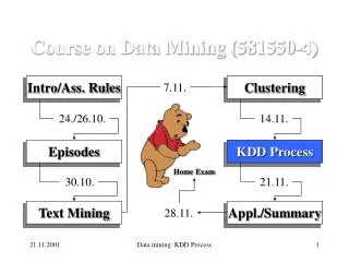
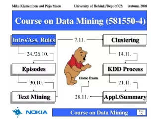
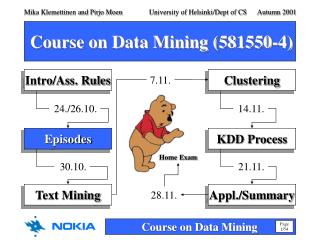
7.11. 24./26.10. 14.11. Home Exam. 30.10. 21.11. 28.11. Course on Data Mining (581550-4). Intro/Ass. Rules. Clustering. Episodes. KDD Process. Text Mining. Appl./Summary. Course on Data Mining (581550-4). Today's subject : Episodes and episode rules Next week's program :

E N D
7.11. 24./26.10. 14.11. Home Exam 30.10. 21.11. 28.11. Course on Data Mining (581550-4) Intro/Ass. Rules Clustering Episodes KDD Process Text Mining Appl./Summary
Course on Data Mining (581550-4) • Today's subject: • Episodes and episode rules • Next week's program: • Lecture: Text mining • Exercise: Episodes and episode rules • Seminar: Episodes and episode rules Today 31.10.2001
Episodes and Episode Rules Basics WINEPI Approach MINEPI Approach Algorithms Examples
Basics • Association rules describe how things occur together in the data • E.g., "IF an alarm has certain properties, THEN it will have other given properties" • Episode rules describe temporal relationships between things • E.g., "IF a certain combination of alarms occurs within a time period, THEN another combination of alarms will occur within a time period"
Network Management System Switched Network MSC MSC MSC BSC BSC BSC Access Network BTS BTS BTS Mobile station controller MSC Base station controller BSC Base station transceiver BTS Basics Alarms
Basics • As defined earlier, telecom data contains alarms: 1234 EL1 PCM 940926082623 A1 ALARMTEXT.. • Now we forget about relationships between attributes within alarms as with the association rules • We just take the alarm number attribute, handle it here as event/alarm type and inspect the relationships between events/alarms Alarm type Date, time Alarm severity class Alarming network element Alarm number
Basics • Data: • Data is a set R of events • Every event is a pair (A, t), where • A R is the event type(e.g., alarm type) • t is an integer, the occurrence timeof the event • Event sequences on R is a triple (s, Ts, Te) • Ts is starting time and Te is ending time • Ts < Te are integers • s = (A1, t1), (A2, t2), …, (An, tn) • Ai R and Ts ti < Tefor all i=1, …, n
D C A B D A B C A D C A B D A 0 10 20 30 40 50 60 70 80 90 100 110 120 130 140 150 Basics • Example alarm data sequence: • Here: • A, B, C and D are event (or here alarm) types • 10…150 are occurrence times • s = (D, 10), (C, 20), …, (A, 150) • Ts (starting time) = 10 and Te (ending time) = 150 • Note: There needs not to be events on every time slot!
Basics • Episodes: • An episode is a pair (V, ) • V is a collection of event types, e.g., alarm types • is a partial order on V • Given a sequence S of alarms, an episode = (V, )occurs within S if there is a way of satisfying the event types (e.g., alarm types) in V using the alarms of S so that the partial order is respected • Intuitively: episodes consist of alarms that have certain properties and occur in a certain partial order
Basics • The most useful partial orders are: • Total orders • The predicates of each episode have a fixed order • Such episodes are called serial (or "ordered") • Trivial partial orders • The order of predicates is not considered • Such episodes are called parallel(or "unordered") • Complicated? • Not really, let's take some clarifying examples
A A A B B B C More complex episode with serial and parallel Serial episode Parallel episode Basics • Examples:
WINEPI Approach • The name of the WINEPI method comes from the technique it uses: a sliding window • Intuitively: • A window is slided through the event-based data sequence • Each window "snapshot" is like a row in a database • The collection of these "snapshots" forms the rows in the database • Complicated? • Not really, let's take a clarifying example
D C A B D A B C 0 10 20 30 40 50 60 70 80 90 WINEPI Approach • Example alarm data sequence: • The window width is 40 seconds, last point excluded • The first/last window contains only the first/last event
event1event2 event3 … … eventn Ts Te t1 t2 t3 … …tn WINEPI Approach • Formally, givena set E of event types an event sequence S = (s,Ts,Te) is an ordered sequence of events eventi such that eventi eventi+1 for all i=1, …, n-1, and Ts eventi < Te for all i=1, …, n
event1event2 event3 … … eventn Ts Te t1 t2 t3 tn WINEPI Approach • Formally, a window on event sequence S is an event sequence S=(w,ts,te), where ts < Te, te > Ts, and w consists of those pairs (event, t) from s where tst < te • The value tst < te is called window width, W ts te W
event1event2 event3 … … eventn Ts Te t1 t2 t3 tn WINEPI Approach • By definition, the first and the last windows on a sequence extend outside the sequence, so that the last window contains only the first time point of the sequence, and the last window only the last time point ts ts te te W W
WINEPI Approach • The frequency (cf. support with association rules) of an episode is the fraction of windows in which the episode occurs, i.e., |Sw W(S, W) | occurs in Sw | fr(, S, W) = |W(S, W)| where W(S, W) is the set of all windows Sw of sequence S such that the window width is W
WINEPI Approach • When searching for the episodes, a frequency threshold (cf. support threshold with association rules) min_fr is used • Episode is frequentif fr(, s, win) min_fr, i.e, "if the frequency of exceeds the minimum frequency threshold within the data sequence s and with window width win" • F(s, win, min_fr): a collection of frequent episodes in s with respect to win and min_fr • Apriori trick holds:if an episode is frequent in an event sequence s, then all subepisodes are frequent
A A B B C : : WINEPI Approach • Formally, an episode rule is as expression , where and are episodes such that is a subepisode of • An episode is a subepisode of ( ), if the graph representation is a subgraph of the representation of
WINEPI Approach • The fraction fr(, S, W) = frequency of the whole episode fr(, S, W) = frequency of the LHS episode is the confidence of the WINEPI episode rule • The confidence can be interpreted as the conditional probability of the whole of occurring in a window, given that occurs in it
WINEPI Approach • Intuitively: • WINEPI rules are like association rules, but with an additional time aspect: If events (alarms) satisfying the rule antecedent (left-hand side) occur in the right order within W time units, then also the rule consequent (right-hand side) occurs in the location described by , also within W time units antecedent consequent [window width] (f, c)
WINEPI Algorithm • Input: A set R of event/alarmtypes, an event sequence s over R, a set E of episodes, a window width win, and a frequency threshold min_fr • Output: The collection F(s, win, min_fr) • Method: 1. compute C1 := { E | || = 1}; 2. i := 1; 3. whileCi do 4.(* compute F(s, win, min_fr) := { Ci | fr(, s, win) min_fr}; 5. i := l+1; 6.(** compute Ci:= { E | || = I, and F||(s, win, min_fr) for all E, }; (* = database pass, (** candidate generation
WINEPI Algorithm • First problem: given a sequence and a episode, find out whether the episode occurs in the sequence • Finding the number of windows containing an occurrence of the episode can be reduced to this • Successive windows have a lot in common • How to use this? • An incremental algorithm • Same idea as for association rules • A candidate episode has to be a combination of two episodes of smaller size • Parallel episodes, serial episodes
WINEPI Algorithm • Parallel episodes: • For each candidate maintain a counter .event_count: how many events of are present in the window • When .event_count becomes equal to ||, indicating that is entirely included in the window, save the starting time of the window in .inwindow • When .event_count decreases again, increase the field .freq_count by the number of windows where remainded entirely in the window • Serial episodes: use a state automata
D C A B D A B C 0 10 20 30 40 50 60 70 80 90 WINEPI Approach • Example alarm data sequence: • The window width is 40 secs, movement step 10 secs • The length of the sequence is 70 secs (10-80)
D C A B D A B C 0 10 20 30 40 50 60 70 80 90 WINEPI Approach • By sliding the window, we'll get 11 windows (U1-U11): … U2 U1 U11 • Frequency threshold is set to 40%, i.e., an episode has to occur at least in 5 of the 11 windows
WINEPI Approach • Suppose that the task is to find all parallel episodes: • First, create singletons, i.e., parallel episodes of size 1 (A, B, C, D) • Then, recognize the frequent singletons (here all are) • From those frequent episodes, build candidate episodes of size 2: AB, AC, AD, BC, BD, CD • Then, recongize the frequent parallel episodes (here all are) • From those frequent episodes, build candidate episodes of size 3: ABC, ABD, ACD, BCD • When recognizing the frequent episodes, only ABD occurs in more than four windows • There are no candidate episodes of size four
WINEPI Approach • Episode frequencies and example rules with WINEPI: D : 73% C : 73% A : 64% B : 64% D A [40] (55%, 75%) D C : 45% D A : 55% D B : 45% D A B [40] (45%, 82%) C A : 45% C B : 45% A B : 45% D A B : 45%
WINEPI: Experimental Results • Data: • Alarms from a telecommunication network • 73 000 events (7 weeks), 287 event types • Parallel and serial episodes • Window widths (W) 10-120 seconds • Window movement = W/10 • min_fr = 0.003 (0.3%), frequent: about 100 occurrences • 90 MHz Pentium, 32MB memory, Linux operating system. The data resided in a 3.0 MB flat text file
Window Serial episodes Parallel episodes width (s) #frequent time (s) #frequent time (s) 10 16 31 10 8 20 31 63 17 9 40 57 117 33 14 60 87 186 56 15 80 145 271 95 21 100 245 372 139 21 120 359 478 189 22 WINEPI: Experimental Results
D C A B D A B C 0 10 20 30 40 50 60 70 80 90 WINEPI Approach • One shortcoming in WINEPI approach: • Consider that two alarms of type A and one alarm of type B occur in a window • Does the parallel episode consisting of A and B appear once or twice? • If once, then with which alarm of type A?
MINEPI Approach • Alternative approach to discovery of episodes • No sliding windows • For each potentially interesting episode, find out the exact occurrences of the episode • Advantages: easy to modify time limits, several time limits for one rule: "If A and B occur within 15 seconds, then C follows within 30 seconds" • Disadvantages: uses a lots of space
MINEPI Approach • Formally, given a episode and an event sequence S, the interval [ts,te] is a minimal occurrence of S, • If occurs in the window corresponding to the interval • If does not occur in any proper subinterval • The set of minimal occurrences of an episode in a given event sequence is denoted by mo(): mo() = { [ts,te] | [ts,te] is a minimal occurrence of }
A A B B C : : D C A B D A B C 0 10 20 30 40 50 60 70 80 90 MINEPI Approach • Example: Parallel episode consisting of event types A and B has three minimal occurrences in s: {[30,40], [40,60], [60,70]}, has one occurrence in s: {[60,80]}
MINEPI Approach • Informally, a MINEPI episode rule gives the conditional probability that a certain combination of events (alarms) occurs within some time bound, given that another combi-nation of events (alarms) has occurred within a time bound • Formally, an episode rule is [win1] [win2] • and are episodes such that ( is a subepisode of) • If episode has a minimal occurrence at interval [ts,te] with te - ts win1, then episode occurs at interval [ts,t'e] for some t'e such that t'e - ts win2
MINEPI Approach • The confidence of the rule [win1] [win2] is the conditional probability that occurs, given that occurs, under the time constraints specified by the rule: |mo()| / |mo()| where |mo()| is the number of minimal occurrences [ts,te] of such that te - ts win1, and |mo()| is the number of such occurrences where there is also an occurrence of within the interval [ts,ts+win2]
D C A B D A B C 0 10 20 30 40 50 60 70 80 90 MINEPI Approach • The frequency of the rule [win1] [win2] is |mo()|, i.e., the number of times the rule holds in the database • Let's take our example data again: • Task: find all serial episodes by using maximum time bound of 40 secs and window sizes 10, 20, 30 and 40 secs. Frequency threshold is set to one occurrence
MINEPI Approach • Find all serial episodes (1/3): • First, create singletons, i.e., episodes of size 1 (A, B, C, D) • While creating the singletons, we also create an occurrence table for them. After this first database pass, we do not have to scan the database anymore, but use the created inverse tables • Then, recognize the frequent singletons (here all are) • From those frequent episodes, build candidate episodes of size 2: AB, BA, AC, CA, AD, DA, BC, CB, BD, DB, CD, DC
MINEPI Approach • Find all serial episodes (2/3): • Then, use the inverse table to create minimal occurrences for the candidates. E.g., for AB take all subepisodes, namely A and B, and compute mo(AB) as follows: • Read the first occurrence of A (30-30), and find the first following B (40-40) • Then take the second occurrence of A (60-60), and find the first following B (70-70) • Then continue with BA
MINEPI Approach • Find all serial episodes (3/3): • In the recognition phase, we find all episodes frequent and build the candidate episodes of size 3. Again, almost all candidates are frequent • Finally, the same procedure is repeated for candidates of size 4, and episodes DCAB in 10-40, DABC in 50-80, CABD in 20-50, CBDA in 20-60, and BDAC in 40-80 are found to occur • Candidates of size 5 are not found, so the algorithm terminates
Minimal (serial) occurrences + frequencies in example data MINEPI Approach
IF D THEN C WITH [0] [10] 0.00 (0/2) [0] [20] 0.50 (1/2) [0] [40] 1.00 (2/2) IF D THEN A C WITH [0] [10] 0.00 (0/2) [0] [40] 0.50 (1/2) IF D A THEN C WITH [40] [40] 0.50 (1/2) [20] [40] 1.00 (1/1) IF D C THEN A B WITH [40] [40] 0.50 (1/2) [30] [40] 1.00 (1/1) MINEPI Approach
IF D A B THEN C WITH [40] [40] 0.50 (1/2) [30] [40] 1.00 (1/1) DAB, DCAB DC DC, DAC, DABC D C A B D A B C 0 10 20 30 40 50 60 70 80 90 DA DA DAB MINEPI Approach • Below are minimal occurrences of the example rules in the example data:
MINEPI: Experimental Results • The same data set as with WINEPI: • Alarms from a telecommunication network • 73 000 events (7 weeks), 287 event types • Serial MINEPI episodes • Time bounds 15-120 seconds • Window movement = W/10 • min_fr = 50-500 • 90 MHz Pentium, 32MB memory, Linux operating system. The data resided in a 3.0 MB flat text file
Min_fr Time bounds (s) 15,30 30,60 60,120 15,30,60,120 50 1131 617 2278 1982 5899 7659 5899 14205 100 418 217 739 642 1676 2191 1676 3969 250 111 57 160 134 289 375 289 611 500 46 21 59 49 80 87 80 138 MINEPI: Experimental Results • Number of episodes and rules:
Min_fr Time bounds (s) 15,30 30,60 60,120 15,30,60,120 50 158 210 274 268 100 80 87 103 104 250 56 56 59 58 500 50 51 51 52 MINEPI: Experimental Results • Execution times:
Summary • Episode rule mining: • Based on association rule techniques • Targeted for temporal data • Two approaches: • WINEPI with a sliding window • MINEPI with the search for minimal occurrences • The approaches can be used for different purposes • In the seminar presentations, we will take a look at… • some other approaches towards sequential pattern mining and • incremental sequential pattern mining
References • Mika Klemettinen, A Knowledge Discovery Methodology for Telecommunication Network Alarm Databases. Report A-1999-1 (PhD Thesis), University of Helsinki, Department of Computer Science, January 1999. ISBN 951-45-8465-1, ISSN 1238-8645. See electronic version at http://www.cs.helsinki.fi/u/mklemett/THESIS/, especially pages 27-49 • H. Mannila, H. Toivonen, and A. I. Verkamo, Discovery of frequent episodes in event sequences, Technical Report C-1997-15, Dept. of Computer Science, University of Helsinki, 1997. See electronic version at http://www.cs.helsinki.fi/research/fdk/datamining/pubs/C-1997-15.ps.gz
Course Organization • Lecture 7.11.: Text mining • Mika gives the lecture • Excercise 8.11.: Episodes and episode rules • Pirjo takes care of you! :-) • Seminar 9.11.: Episodes and episode rules • Mika gives the lecture • 2 group presentations Next Week