Download
1 / 56
610 likes | 829 Vues
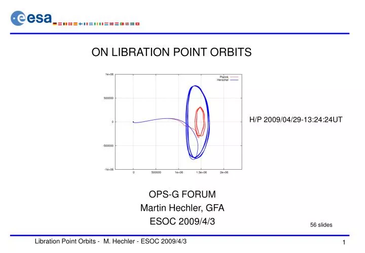
ON LIBRATION POINT ORBITS . H/P 2009/04/29-13:24:24UT. OPS-G FORUM Martin Hechler, GFA ESOC 2009/4/3. 56 slides. Contents. Lagrange points in Sun-Earth system and orbits around them ESA missions at L 2 and L 1 (Sun-Earth): Why there ? In which orbits ?

E N D
ON LIBRATION POINT ORBITS H/P 2009/04/29-13:24:24UT OPS-G FORUMMartin Hechler, GFAESOC 2009/4/3 56 slides Libration Point Orbits - M. Hechler - ESOC 2009/4/3
Contents • Lagrange points in Sun-Earth system and orbits around them • ESA missions at L2 and L1 (Sun-Earth): Why there ? In which orbits ? • From basics of linear theory to numerical orbit construction • Transfers to L2 or L1 : Stable manifold and weak stability boundary • The freely reachable orbits (Herschel, JWST) • Transfer optimisation to Lissajous orbits (Planck, GAIA) • Launch windows (Herschel/Planck, GAIA) • Lunar flybys, transfers with apogee raising sequence (LISA pathfinder) • Navigation: orbit determination and orbit correction manoeuvres Libration Point Orbits - M. Hechler - ESOC 2009/4/3
Libration Points Orbits at L2 Missions Going there Libration Point Orbits - M. Hechler - ESOC 2009/4/3
Libration Points in Sun-Earth • Libration Points: • 5 Lagrange Points • L1 and L2 of interest for space missions Lagrange 1736-1813 • Satellite in L2: • Centrifugal force (R=1.01 AU) balances central force (Sun + Earth) • 1 year orbit period at 1.01 AU with Sun + Earth attracting • Satellite remains in L2 • However: Theory of Lagrange only valid if Earth moves on circle and Earth+Moon in one point • But orbits around L2 exist Libration Point Orbits - M. Hechler - ESOC 2009/4/3
Orbits at L2 y Satellite in L2 • Does notwork in exact problem • Would also be in Earth half-shadow • And difficult to reach (much propellant) Satellites in orbits around L2 • With certain initial conditions a satellite will remain near L2 also in exact problem called Orbits around L2 • Different Types of Orbits classified by their motion in y-z (z=out of ecliptic) x Libration Point Orbits - M. Hechler - ESOC 2009/4/3
Orbit Families at Libration Points • ‘Strict’ Halo orbits: • ‘quasi periodic’: z-frequency = x-y-frequency • large amplitudes (AY ≥ 600000 km) • loss of one degree of freedom in initial state • in general no free transfer • free of eclipse by definition • Quasi Halo orbits: • not periodic • free transfer possible, stable manifold “touches” launch conditions • can be free of eclipse for long time • Lissajous orbits: • small amplitude possible • large insertion ∆V • can be free of eclipse for 6 years • condition on initial state Libration Point Orbits - M. Hechler - ESOC 2009/4/3
Criteria for Selection of Orbit Class at L2 • No essential advantage of ‘strict’ Halos • Orbit selection on mission requirements alone • Typical selection criteria: • no eclipse • limit on sun-spacecraft-Earth angle e.g. for communication system design • ∆V budget • Two families of orbits of most interest • Minimum transfer ∆V Quasi-Halos • Lissajous orbits without eclipse for 6 years Libration Point Orbits - M. Hechler - ESOC 2009/4/3
Why do Astronomy Missions go to L2 ? • Advantages for Astronomy Missions: • Sun and Earth nearly aligned as seen from spacecraft • stable thermal environment with sun + Earth IR shielding • only one direction excluded form viewing (moving 360o per year) • possibly medium gain antenna in sun pointing • Low high energy radiation environment • Drawbacks: • 1.5 x 10⁶ km for communication • However development of deep space communications technology (X-band, K-band) ameliorates this disadvantage • Long transfer duration Fast transfer in about 30 days with +10 m/s • Instable orbits frequent manoeuvres, escape in case of problems and at end of mission (L2 region “self-cleaning”) Libration Point Orbits - M. Hechler - ESOC 2009/4/3
Used Orbit Classes for Missions at L1 and L2 • Lissajous orbits: • Earth aspect <15o • Survey Missions • scanning in • sun pointing spin • Quasi Halo orbits: • “Free” transfer • Observatories View from Earth Herschel JWST LISA Pathfinder (L1) XEUS EUCLID PLATO SPICA Planck GAIA Libration Point Orbits - M. Hechler - ESOC 2009/4/3
ESA Missions to L2 (and L1) Libration Point Orbits - M. Hechler - ESOC 2009/4/3
Herschel + Planck Libration Point Orbits - M. Hechler - ESOC 2009/4/3
GAIA Libration Point Orbits - M. Hechler - ESOC 2009/4/3
ESA Missions to L2 in Planning Phase Libration Point Orbits - M. Hechler - ESOC 2009/4/3
From Linear Theory to Numerical Orbit Construction Libration Point Orbits - M. Hechler - ESOC 2009/4/3
Basics: Linear Theory of Orbits at L2 (1) Circular restricted problem Libration Point Orbits - M. Hechler - ESOC 2009/4/3
Basics: Linear Theory of Orbits at L2 (2) Lis-ELEVEC AND Lis-VECELE (for t=0) : Ax= 1/c2 Ay Fast variables Libration Point Orbits - M. Hechler - ESOC 2009/4/3
Basics: Linear Theory of Orbits at L2 (3) Libration Point Orbits - M. Hechler - ESOC 2009/4/3
Basics: Linear Theory of Orbits at L2 (4) • Exact problem inherits properties from linear problem • Use ∆V-direction of linear problem in numerical method Libration Point Orbits - M. Hechler - ESOC 2009/4/3
Exact Problem: Unstable Manifold Orbits at L2 are unstable escape for small deviation generates unstable manifold e+λt x-y rotating = in ecliptic Sun-Earth on x-axis To solar system Libration Point Orbits - M. Hechler - ESOC 2009/4/3
Outward Escape on Unstable Manifold 1 m/s 10 cm/s 10 m/s 1 revolution ≈ 180 days Libration Point Orbits - M. Hechler - ESOC 2009/4/3
Inward Escape on Unstable Manifold -10 cm/s -1 m/s -10 m/s Libration Point Orbits - M. Hechler - ESOC 2009/4/3
Central Manifold No escape +10 cm/s -10 cm/s Libration Point Orbits - M. Hechler - ESOC 2009/4/3
Stable Manifold of HERSCHEL Orbit “Stable manifold” = surface-structure in space, which flows into orbit Herschel orbit Transfer Perigee of stable manifold Of Herschel Orbit e-λt Libration Point Orbits - M. Hechler - ESOC 2009/4/3
Stable Manifold of PLANCK Orbit Planck orbit Transfer Jump onto stable manifold e-λt Perigee of stable manifold of Planck Orbit Libration Point Orbits - M. Hechler - ESOC 2009/4/3
Stable Manifold and Weak Stability Boundary Backward Forward • Weak Stability Boundary: • Perigee from launch conditions (i, Ω, ω) • Scan and bisection in perigee velocity (Vp) • One non escape solution (free transfer) • Transfers to Quasi-Halos • Stable Manifold: • Backward integration from orbit at L1/2 • “Jump onto stable manifold” • Two local minima in ΔV (fast/slow) • Used for transfers to “constrained” orbits fast Example bisection slow Libration Point Orbits - M. Hechler - ESOC 2009/4/3
Example Bisection in Perigee Velocity Integrate until > 2000000 km or < 800000 km Bisection in velocity bisec dv(m/s) days rstop(km) 0 3.013107155600253 103.5 855325.3 0 4.013107155600253 119.7 2319036.2 0 3.513107155600253 140.6 2044164.8 1 3.263107155600253 137.6 1094563.3 2 3.388107155600254 160.1 2070930.6 3 3.325607155600254 213.0 827084.2 4 3.356857155600254 174.8 2080976.5 5 3.341232155600254 193.6 2052903.9 6 3.333419655600254 293.1 2324254.3 7 3.329513405600254 230.4 801319.6 8 3.331466530600254 248.6 828429.7 9 3.332443093100254 272.2 825422.6 10 3.332931374350254 321.7 2019561.9 11 3.332687233725253 291.1 859153.3 12 3.332809304037754 346.9 1158669.1 13 3.332870339194003 338.0 2084535.5 14 3.332839821615878 364.8 2092294.5 15 3.332824562826816 384.0 870165.7 16 3.332832192221348 450.0 2280789.3 To Earth To Sun 2 revolutions “Non-escape” if >450 days Stop box 1 mm/s ≈ 1% of radiation pressure effect over 10 days Computer word length Integrator accuracy mm/s ≈ orbit determination accuracy ≈ dynamic noise Libration Point Orbits - M. Hechler - ESOC 2009/4/3
Numerical Construction of Orbits to/at L2 • Same procedure from any point in orbit • Initial guess of state • from forward integration of transfer • or from analytic theory • Correction of velocity by scan + bisection along escape direction u • Integrate e.g. 1/2 revolution and repeat forward process • “Mathematical” ∆V’s ≈ 1 mm/s per revolution (far below navigation ∆V) • No gradients, no terminal conditions (only non-escape) • Orbit construction based on Weak Stability Boundary method Libration Point Orbits - M. Hechler - ESOC 2009/4/3
Non-gravitational Accelerations • No difference for orbit generation method if other deterministic perturbations • are included in dynamics: • Radiation pressure (may be lifting – GAIA) • attitude manoeuvre effects, if predictable • wheel off-loading (may be used to correct orbit – Herschel) • large known manoeuvres • Weak Stability Boundary Orbit Construction Method • also works for perturbed gravity field Libration Point Orbits - M. Hechler - ESOC 2009/4/3
Orbit with 10 x Radiation Pressure Shift towards sun Libration Point Orbits - M. Hechler - ESOC 2009/4/3
HERSCHEL Orbit (Halo) 4 years propagation Launch 2009/4/29 – 13:24:24 Remark: For the nominal launch time the Herschel orbit is nearly a Halo (by chance) Libration Point Orbits - M. Hechler - ESOC 2009/4/3
PLANCK Orbit (Lissajous) 2.5 years propagation Libration Point Orbits - M. Hechler - ESOC 2009/4/3
Navigation and Orbit Maintenance later Transfer Optimisation and Launch Windows Libration Point Orbits - M. Hechler - ESOC 2009/4/3
Result: Optimum Planck Transfer Herschel “free” transfer Planck ≠ Herschel from day 2 Libration Point Orbits - M. Hechler - ESOC 2009/4/3
Transfer Optimisation (Planck/GAIA) Herschel/Planck: (i, ω, Vp, Tp~Ω) all fixed GAIA: ω and Ω free Solved by forward/backward shooting Cost functional (Σ║ΔV║=min) Departure variables launch (i, Ω, ω, Vp, Tp) Arrival variables Lissajous (Ay,Az,Фz,Ty=0) With prescribed properties: (α < 15o and no eclipse) Tp Day 2 Tm Fast Transfer: Ti – Tp < 50 days Ti Matching constraint (ΔX=0) Number of manoeuvres depends on case Libration Point Orbits - M. Hechler - ESOC 2009/4/3
Planck Manoeuvre Model • All manoeuvres are done in sun pointing mode • Decomposition modelled in optimisation • ΔV of each thruster + phase angle (5 variables) • ║ΔV║ = sum of ΔV’s of thrusters ~ propellant • Optimisation in general converges to “pure manoeuvres” Libration Point Orbits - M. Hechler - ESOC 2009/4/3
Launch Windows • Definition of Launch Window: • Dates (seasonal) and hours (daily) for which a launch is possible • “Best” launcher target conditions (possibly as function of day and hour) • Constraints: • Propellant on spacecraft required to reach a given orbit (type) • Geometric conditions: • eclipses • sun aspect angles Typical method: • Calculate orbits for scan in launch times • shade areas for which one of the conditions is not satisfied Libration Point Orbits - M. Hechler - ESOC 2009/4/3
Herschel/Planck Launch Window: Vp Selection • Double launch on ARIANE 5: rp, i, ω for maximum mass • Fixed launch conditions in Earth fixed frame at lift-off • only one flight program on launcher (cost saving) • Vp to be fixed • Both spacecraft correct perigee velocity Vp (~ ra) • Fast transfer vp about 2 m/s below vp of stable manifold • Launch conditions of Ariane: • Vp = Vesc - 30.32 m/s • Ra = 1 200 000 km 4/29 J2 corrected • Osculating at Planck S/C separation • J2 must be on in integration Remaining degree of freedom: Ω Libration Point Orbits - M. Hechler - ESOC 2009/4/3
Herschel/Planck Launch Window (as of 2007) • 140 launch orbit Libration Point Orbits - M. Hechler - ESOC 2009/4/3
Herschel/Planck Launch Window (as of 2008) • 60 launch orbit Libration Point Orbits - M. Hechler - ESOC 2009/4/3
Herschel/Planck Launch Window (now) • 60 launch orbit • Both S/C tanks full • Change of launcher • axis at fairing separation • 15 min lost 4/29 Launch window on 2009/4/29: 13:24:24 – 14:06:24 UT Libration Point Orbits - M. Hechler - ESOC 2009/4/3
GAIA Seasonal Launch Window • Soyuz from French Guyana to circular parking orbit at 15o inclination • 2nd Fregat burn at any time in circular orbit to reach L2 transfer (free ω) • Two degrees of freedom (Ω, ω) optimum transfer near ecliptic plane 165 m/s One optimum launch time per day Libration Point Orbits - M. Hechler - ESOC 2009/4/3
GAIA Fast Transfer to L2 and 6 Years Orbit • Cycle eclipse to eclipse > 6 years • choice of initial z-phase Libration Point Orbits - M. Hechler - ESOC 2009/4/3
Transfer with Lunar Gravity Assist • Perigee of stable manifold of small amplitude Lissajous orbits above 50000 km • Intersects Moon orbit at two points → two solutions from Moon to given orbit Cross section Launch orbit near lunar orbit plane Libration Point Orbits - M. Hechler - ESOC 2009/4/3
Lunar Flyby Opportunities + Phasing • One opportunity per month • Earth to moon 2-3 days Navigation difficult • Necessity of phasing orbits • Launch to orbit below moon (200000 km) • Sequence of apogee raising manoeuvres • Also perigee raising manoeuvres necessary against perturbations • Launcher dispersion correction with manoeuvres at perigee Libration Point Orbits - M. Hechler - ESOC 2009/4/3
L2 Transfer with Lunar Gravity Assist • Currently discussed again for Baikonur back-up Libration Point Orbits - M. Hechler - ESOC 2009/4/3
LISA Pathfinder Apogee Raising Sequence • Large liquid propulsion stage (440 N, 321 s) connected to S/C • ~15 manoeuvres at perigee to raise apogee from 900 km to 1.3 x 10⁶ *km (to L1) • Gravity loss limited to 1.5% (in total ΔV) Example case above for old Rockot launch scenario Libration Point Orbits - M. Hechler - ESOC 2009/4/3
Navigation and Orbit Maintenance Libration Point Orbits - M. Hechler - ESOC 2009/4/3
Recovery from Escape due to Noise Extreme example • Unknown random accelerations or events perturb orbit • S/C will move away on unstable manifold (in or out) • Orbit Maintenance necessary back on stable manifold of another non-escape orbit 20 m/s 30 days 65 m/s Cost increases with delay Libration Point Orbits - M. Hechler - ESOC 2009/4/3
Navigation Process Real World Random number Execution error Noise Manoeuvre Execution XRW Dynamics XRW Errors Measurements ∆V z Ground System State extended By noise model parameters Orbit Determination Manoeuvre Optimisation Measurements Model Estimation XEST Objective = no escape Dynamics Model with noise model XEST Libration Point Orbits - M. Hechler - ESOC 2009/4/3
Navigation Mission Analysis Real World Simulation Noise Random numbers Execution error Random numbers Manoeuvre Execution xsim Dynamics Model xsim Errors Random Numbers Measurements Model Monte-Carlo |∆V| sampling ∆V z Ground System Representation OD + Covariance analysis Manoeuvre Optimisation Measurements Model Estimation Filter x, C Objective = no escape Dynamics Model with noise model x, C Knowledge Covariance Libration Point Orbits - M. Hechler - ESOC 2009/4/3