Download

1 / 21
210 likes | 447 Vues
Chapter 4 Roots of Polynomials. Objectives. Understand the importance of finding polynomial roots in engineering applications Know the conventional method concept Know the Muller’s method concept Know the Bairstow’s method. Content. Polynomials in engineering and science

E N D
Chapter 4 Roots of Polynomials
Objectives • Understand the importance of finding polynomial roots in engineering applications • Know the conventional method concept • Know the Muller’s method concept • Know the Bairstow’s method
Content • Polynomials in engineering and science • Conventional method • Muller’s method • Bairstow’s method • Conclusions
Polynomials in… (1) General solutions of linear ODE Solve for general solution Change to characteristic equations: The results can be :-
Polynomials in…(2) General solutions of linear ODE
Polynomials in…(3) • Problem : • Follow these rules: • For an nth order equation, there are n real or complex roots. • If n is odd, there is at least one real root. • If complex roots exist, they will be in conjugate pairs (that is, l+mi and l-mi), where i=sqrt(-1).
Conventional… • Only real roots exist However, • Finding good initial guesses complicates both the open and bracketing methods, also the open methods could be susceptible to divergence. • Real and complex roots of polynomials – Müller and Bairstow methods.
Müller method (1) • Like Secant, Müller’s method obtains a root estimate by projecting a parabola to the x axis through three function values.
Müller method (2) Secant method (linear approximation)
Müller method (3) Müller method (Parabola or 2nd order approximation) Must use three points to approximate function
Müller method (4) Müller methodology derivation • Write the equation in a convenient form at point x2: • We then have three eqns now (from x0, x1, and x2)
Müller method (5) • Step III Reduce to two eqns Right now u can solve for a and b from When u know a, b, c you are ready to estimate root from
Müller method (6) • Step IV Here the new estimated root is Two roots, but which one ? • Error can be derived from
Müller method (7) • Summary of algorithm Start with 3 points [x0,f(x0)] [x1,f(x1)] and [x2,f(x2)] Calculate a, b, and c from
Müller method (8) • Summary of algorithm (cont’d) Calculate new root from Calculate error Check whether new xi-1 = old xi
Bairstow’s method (1) • An iterative approach loosely related to both Müller and Newton Raphson methods. • Based on dividing a polynomial by a factor x-t: Start with Dividing with x-t yields and a remainder R=b0 The coefficients of polynomial are
Bairstow’s method (2) • To permit the evaluation of complex roots, Bairstow’s method divides the polynomial by a quadratic factor x2-rx-s: For the remainder to be zero, boand b1 must be zero. However, it is unlikely that our initial guesses at the values of r and s will lead to this result, so we do this…
Bairstow’s method (3) Using a similar approach to Newton Raphson method, both bo and b1can be expanded as function of both r and s in Taylor series. Neglect higher-order terms We estimate Δr and Δs from How can we find these partial derivatives ???
Bairstow’s method (4) Partial derivatives can be obtained by a synthetic division of the b’s in a similar fashion the b’s themselves are derived: where then
Bairstow’s method (5) At each step, the error can be estimated as The roots can be determined from
Bairstow’s method (6) • At this point three possibilities exist: • The quotient is a third-order polynomial or greater. The previous values of r and s serve as initial guesses and Bairstow’s method is applied to the quotient to evaluate new r and s values. • The quotient is quadratic. The remaining two roots are evaluated directly, using • The quotient is a 1st order polynomial. The remaining single root can be evaluated simply as x=-s/r.