Download
1 / 13

E N D
NOAA High Impact Weather Working Group Workshop, Norman, OK, 24 Feb 2011Tropical Cyclone/Hurricane Data Assimilation: An Ensemble Data Assimilation viewMilija ZupanskiCooperative Institute for Research in the AtmosphereColorado State UniversityFort Collins, Colorado, U. S. A.[ http://www.cira.colostate.edu/projects/ensemble/ ] Acknowledgements: - NOAA HFIP, NCEP/EMC - JCSDA/NESDIS - NASA PMM
TC/Hurricane data assimilation • Remote sensing is a major source of information - radar data - satellite data • Data assimilation has to be able to efficiently utilize these data - cloudy/precipitation-affected radiances - nonlinear transformation from model to observations (observation operators) • Localized phenomenon • - dynamical impact on error covariances • - relevance of microphysics • Challenges • - improving intensity and position • - new instruments (e.g. GOES-R GLM, ABI) • - hyper-spectral (thousands of channels) • - large number of observations (e.g., cloudy radiances, hyperspectral sounders)
Remote sensing data coverage Radar Reflectivity AMSU-A GOES-11 SNDR • Radar data are typically available only over land - coastal areas - airborne/spaceborne radars - almost continuous spatiotemporal coverage • Satellite data are available everywhere - open ocean - intermittent coverage (e.g. geostationary vs. polar-orbiting) Combined use of all data is best choice
First guess - dynamically relevant, high resolution, best forecast (easier to adjust good forecast than bad forecast) - also used for error covariance calculation (EnsDA) • Forecast error covariance - need to reflect true uncertainties of TC forecast - geographically localized in the area of storm - correlated control variables (e.g. dynamics, microphysics) • Utilize remote sensing observations • - impact on intensity and position (e.g., IR, MW radiances) • - cloudy radiance assimilation (TC is “defined” by clouds) • - nonlinear analysis solution • Improve TC intensity and position • - microphysical control variables • - focus on improving the forecast after DA • - include new instruments (e.g. GOES-R GLM, ABI) • Uncertainty estimation • - TC forecast uncertainty important as an input for decision-making Relevant components of TC data assimilation
Correct DA impact Incorrect DA impact No DA impact Obs increments [y-H(x)] Obs increments [y-H(x)] Obs increments [y-H(x)] Forecast uncertainty (Pf) Forecast uncertainty (Pf) Forecast uncertainty (Pf) What is DA actually doing? • It projects observation increments to a subspace defined by forecast error covariance Recall the KF analysis equation where The forecast error covariance is The analysis increment becomes Analysis increment is a linear combination of Pfbasis vectors (U) • (1) Analysis increment will be non-zero if • (2) This implies that the range of Pfis critical for creating good analysis
V-wind U-wind t=0 h (3-d Var) t=3 h (4-d Var) U-wind Rain Ice V-wind Forecast error covariance Analysis response to a single U-wind obs near surface Variational error covariance Ensemble error covariance (EnsDA, t=3 h) • symmetric at initial time (3-d Var) • changed by model at end time (4-d Var) • only for basic model variables (p,T,u,v,q) • similar to variational in horizontal • strong dynamical response in vertical • response of microphysical variables
Impact of cloud clearing (radiance assimilation) TC Gustav (2008): RMS errors with respect to observed AMSU-B radiances. Time coverage indicates that only 1/3 of data assimilation cycles (6 out of 18 in this example) had available radiance observations. Re-development of the TS Erin (2007): Distribution of AMSU-B radiance data in the NCEP operational data stream: (a) all observations, (b) accepted observations after cloud clearing. Data are collected during the period 15-18Z, August 18, 2007. Note that almost all observations in the area of the storm got rejected by the cloud clearing. (from Zupanski et al. 2011, J. Hydrometeorology) Need assimilation of all-sky radiances (improve observation information value)
Nonlinear observation operators • Transformation from forecast model variables to radiance is complex - need not only spatial interpolation but also radiative transfer - computational overhead • Nonlinearities increase for precipitation affected radiances - absorption and scattering - clouds, aerosol • Most EnsDA methods use (linear) Kalman filter analysis solution (K operator assumed linear in KF) • Variational DA and some EnsDA methods use an iterative nonlinear minimization of a cost function
COV QSNOW, QSNOW COV QSNOW,QRAIN No cloud ice adjustment With cloud ice adjustment 5-10 K > 25 K COV QSNOW, V-wind Analysis increment of at 850 hPa Relevance of microphysics control variables • TC intensity - microphysical processes are fundamental for TC intensity forecast - need adjustment of microphysics control variables in DA (in addition to dynamics) Microphysics control variables: forecast error covariance structure Microphysics control variables: impact on DA Physically unrealistic analysis adjustment without microphysics control variable (cloud ice in this example)
Degrees of Freedom for Signal • Measure of DA efficiency/value - important indicator of DA performance • Sub-optimal in both variational DA and EnsDA methods due to sub-optimal forecast error covariance - full-rank, but static, modeled function in Var DA - situation-dependent, dynamical, but reduced-rank in EnsDA where C is the observation information matrix (Rodgers, 2000; Zupanski et al. 2007, QJRMS) Degrees of Freedom for Signal (DFS, Rodgers 2000):
Wind analysis uncertainty (500 hPa) Degrees of Freedom for Signal (DFS) OBS 89v GHz Tb METEOSAT Imagery valid at 19:12 UTC 18 Jan 2007 Cloud ice analysis uncertainy Degrees of Freedom for Signal (DFS) all-sky radiance observation information content MW radiances: AMSR-E data assimilation (Erin, 2007) (from Zupanski et al. 2011, J. Hydrometeorology) IR radiances: Assimilation of synthetic GOES-R ABI (10.35 mm) all-sky radiances (Kyrill, 2007) (from Zupanski et al. 2011, Int. J. Remote Sensing) Analysis uncertainty and DFS are flow-dependent, largest DFS in cloudy areas of the storm.
Surface precipitation short-term forecasts verification Accumulated rain during 15-22 September 2009 in the Southeast flood region Ground-based Verification (NOAA Stage IV data) 3DVAR, WRF-GSI (no AMSR-E, TMI) EnsDA, WRF-EDAS (with AMSR-E, TMI) Assimilation of precipitation-affected radiance improves short-term precipitation forecasts, in spatial pattern and intensity - implications to TC/hurricane DA
Summary • Cloudy radiance assimilation is required for improved analysis • Forecast error covariance needs to be state-dependent, and also to represent dynamical and microphysical correlations • Microphysics control variables should benefit TC analysis (e.g. intensity) • Nonlinear analysis capability required • DFS may be important for measuring progress of DA • Combination of observations from various sources is needed (IR radiance is good for TC track, MW for TC intensity) • Observations from new instruments/platforms (for example, GOES-R GLM is related through microphysics, impacts both track and intensity) • Analysis/forecast uncertainty estimation is required for decision-making