Download
1 / 92
970 likes | 1.38k Vues
Ensemble Prediction System (EPS) - ECMWF. With contributions from : Roberto Buizza, Martin Leutbecher, David Richardson, Gerald van der Grijn and others. Ervin Zsoter ECMWF, Meteorological Operations Section ervin.zsoter@ecmwf.int. Flow dependence of forecast errors. Control D-1.

E N D
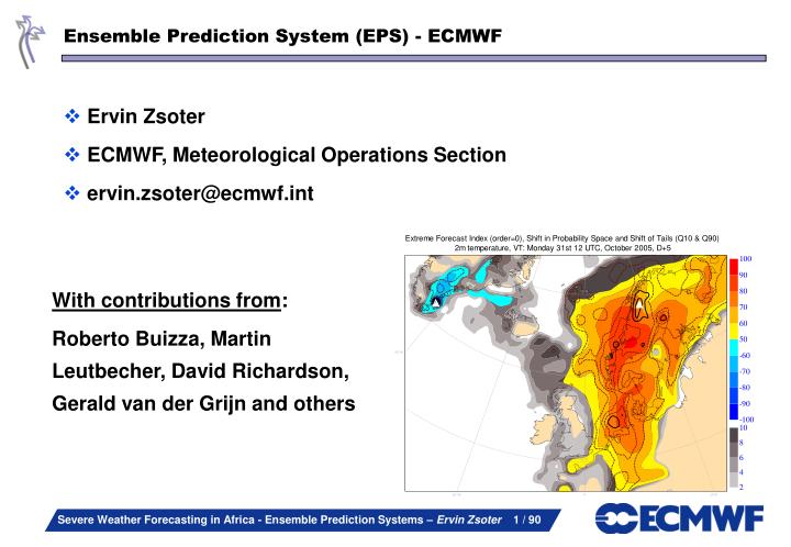
Ensemble Prediction System (EPS) - ECMWF With contributions from: Roberto Buizza, Martin Leutbecher, David Richardson, Gerald van der Grijn and others Ervin Zsoter ECMWF, Meteorological Operations Section ervin.zsoter@ecmwf.int
Flow dependence of forecast errors Control D-1 Control D-1 26th June 1995 26th June 1994 Forecasters have long learned to adjust their forecast with their experience of model errors (flow dependence, forecast range dependency) Inconsistency of the forecasts (between different runs or between different models) were used as indication of the (un-) predictability of scenarios Need for a tool that provide an explicit, detailed representation of model uncertainties, and potential of unusual events
Sources of forecast errors: initial and model uncertainties Weather forecasts lose skill because of the initial condition uncertainties • Observation errors (observations have a finite precision, point observations may not be very representative of what happens inside a model grid box). • Imperfect boundary conditions (e.g. roughness length, soil moisture, snow cover, vegetation properties, sea surface temperature). • Data assimilation assumptions (e.g. relative weights given to observations, statistics). And because of numerical model errors • e.g. due to a lack of resolution, simplified parameterization of physical processes, arbitrariness of closure assumptions, the effect of unresolved processes. As a further complication, predictability (i.e. error growth) is flow dependent • Small uncertainties grow to large errors (unstable flow) • Small scale errors will affect the large scale (non-linear dynamics) • “Does the Flap of a Butterfly’s Wings in Brazil set off a Tornado in Texas?” Ed Lorenz, 1972 Lorenz 3D chaos model
The atmosphere exhibits a chaotic behavior: an example MSLP ensemble forecast of the French/German storm (Lothar), Start date 24 Dec 1999 FT: T+42h A dynamical system shows a chaotic behavior if most trajectories exhibit sensitivity to initial conditions, i.e. if most trajectories that pass close to each other at some point do not remain close as time progresses. This figure shows the high resolution deterministic forecast, the verifying analysis (top-left) and 50 +42h forecasts of mean-sea-level pressure started from slightly different initial conditions (i.e. from initially very close points, see on the bottom). T+0h T+0h EPS member 13 EPS member 14
Predictability is flow dependent: spaghetti plots The degree of clustering of Z500 isolines is an index of low/high perturbation growth (and predictability or uncertainty). small uncertainty large uncertainty
Temperature Temperature fcj fc0 PDF(t) reality PDF(0) Forecast time The probabilistic approach to NWP: What is an ensemble prediction? A complete description of the weather prediction problem can be stated in terms of the time evolution of an appropriate probability density function (PDF) which gives a range of future weather scenarios consistent with our knowledge of the initial state and model capability • Provides explicit indication of uncertainty in today’s forecast Ensemble prediction based on a finite number of deterministic integration appears to be the only feasible method to predict the PDF beyond the range of linear growth. A set of forecasts run from slightly different (perturbed) initial conditions to account for initial uncertainties
Evolution of the PDF T=0h T=72h T=144h
What does it mean to ‘predict the PDF time evolution’? The ensemble spread around the control forecast can be used to identify areas of potential large control-forecast error. These figures show the 5-day control forecast and ensemble spread (left) and the verifying analysis and the control error (right) for forecasts started 18 January 1997 (top) and 1998 (bottom).
What should an ensemble prediction system simulate? What is the relative contribution of initial conditions and model uncertainties to forecast error? Richardson (1998, QJRMS) has compared forecast runs with two models (UK and ECMWF) starting from either UK or ECMWF initial conditions (ICs). Results indicated that initial differences explains most of the differences between ECMWF-from-ECMWF-ICs and UK-from-UK-ICs forecasts.
What should an ensemble prediction system simulate? • This figure shows the difference between 3 5-day forecasts: • UK(UK) (i.e. UK-from-UK-ICs) and EC(EC) (top left) • EC(UK) and EC(EC) (top right) • UK(UK) and EC(UK) (bottom left) • The error of the EC(EC) forecast is also shown (bottom left) • It can be seen that initial differences contribute more than model differences to forecast divergence. This suggests that initial uncertainties contributes more than model approximations to error growth during the first 3-5 forecast days. • How should an ensemble system simulate the uncertainty in the ICs ?
There is a strong constraint: limited resources (man and computer power) What should an ensemble prediction system simulate? Two schools of thought: • Monte Carlo approach: sample all sources of forecast error. Rationale: perturb any input variable (observations, boundary fields, …) and any parameter that is not perfectly known. Take into consideration as many sources as possible of forecast error. • Reduced sampling: sample leading sources of forecast error (prioritize). Rationale: due to the complexity and high dimensionality of the system properly sampling the leading sources of errors is crucial. Rank sources, prioritize, optimize sampling: growing components will dominate forecast error growth.
Simulation of initial uncertainties: selective sampling At theMeteorological Service of Canada MSC, the perturbed initial conditions are generated by running an ensemble of assimilation cycles that use perturbed observations and different models (Monte Carlo approach). At ECMWF and National Centers for Environmental Predictions (NCEP) the perturbed initial conditions are generated by adding perturbations to the unperturbed analysis generated by the assimilation cycle. The initial perturbations are designed to span only a subspace of the phase space of the system (selective sampling). These ensembles do not simulate the effect of imperfect boundary conditions.
t=T2 t=T1 t=0 Selective sampling: singular vectors (ECMWF) Perturbations pointing along different axes in the phase-space of the system are characterized by different amplification rates. As a consequence, the initial PDF is stretched principally along directions of maximum growth. The component of an initial perturbation pointing along a direction of maximum growth amplifies more than components pointing along other directions. At ECMWF, maximum growth is measured in terms of total energy and a perturbation time evolution is linearly approximated. The adjoint of the tangent forward propagator with respect to the total-energy norm is defined, and the singular vectors, i.e. the fastest growing perturbations, are computed by solving an eigenvalue problem.
How is it produced – Singular vectors 1st Singular Vector (Temperature perturbation, 18 Jan 1997, lat=36N) t=0 • SV have a strong baroclinic tilt at initial time (but lose it over 48h – non-normal modes) • SV propagate downflow t=+48h
Kinetic How is it produced – Singular vectors The top figure shows the SV1:25 average vertical distribution at initial time of the kinetic (red dotted, x100) and total (red solid, x100) energy, and the corresponding final time distributions (blue). The bottom figure shows the SV1:25 average total energy spectrum at initial (red solid, x100) and at final time (blue solid). Note the SV typical upward and upscale energy transfer/growth, and the transformation from initial potential to mainly final kinetic energy. t=0 (*100) t=+48h
Selective sampling: breeding vectors (NCEP) At NCEP a different strategy based on perturbations growing fastest in the analysis cycles (bred vectors, BVs) is followed. The breeding cycle is designed to mimic the analysis cycle. Each BV is computed by (a) adding a random perturbation to the starting analysis, (b) evolving it for 24-hours (soon to 6), (c) rescaling it, and then repeat steps (b-c). BVs are grown non-linearly at full model resolution.
Definition of the perturbed ICs NH SH TR Products 1 2 50 51 ….. The current ECMWF Ensemble Prediction System The Ensemble Prediction System (EPS) consists of 51 10-day forecasts run at resolution TL399L62 (~60km, 62 levels) [1,5,7,8,13,11,15]. The EPS is run twice a-day, at 00 and 12 UTC. Initial uncertainties are simulated by perturbing the unperturbed analyses with a combination of T42L62 singular vectors, computed to optimize total energy growth over a 48h time interval (OTI). • Uses the same tangent-linear and adjoint models as used for the 4D-Var analysis 50 perturbations are generated by random (Gaussian) sampling from 50 singular vectors (each perturbation is a weighted combination of all the 50 singular vectors). Amplitude of singular vectors are tuned so that their local maxima are comparable to local analysis errors and to have a realistic ensemble spread after 48 hours Evolved singular vectors from 48 h earlier are also used
20040315 12UTC ECMWF EPS Cont FC t+ 0 VT: 20040315 12UTC 700z 1000 20 13 8 5 3 2 Conventional EPS perturbations are mainly acting on the extra-tropics The conventional EPS lacks initial perturbations in the tropical region and will for this reason not inform optimally about probable future states of the atmosphere for this region. Consequently, it will not perform optimally in areas in the mid-latitudes that are influenced by certain tropical regions (e.g. tropical cyclones). Initial EPS perturbations of geopotential at 700hPa
Targeted Tropical Perturbations Before September 2004, tropical singular vectors (TR-SVs) were computed inside areas with northern boundary with 25°N: this was causing an artificial ensemble-spread reduction when tropical cyclones were crossing 25°N. Furthermore, TR-SVs were computed only if WMO cl-2 TC were detected between 25°S-25°N, and too few tropical areas (up to 4) were considered. On 28 Sep ‘04, a change was introduced to address this issue. In the new system: • Targeted areas extend north of 30°N, and are defined considering the predicted TCs’ tracks • Up to 6 areas can now be targeted • Tropical depression (WMO cl1) detected between 40°S-40°N are targeted • SVs are computed using a new ortho-normalization procedure • Overlapping areas are merged • Caribbean are included (0-25N, 100-60W) if no TC in area
Reliability diagram for strike probabilities Old CY28R2 EPS New CY28R3 EPS TR-SVs’ target areas: impact of the Sep ’04 change Results based on 44 cases (from 3 Aug to 15 Sep 2004) indicate that the implemented changes in the computation of the tropical areas has a positive impact on the reliability diagram of strike probability.
‘Stochastic physics’ and the ECMWF EPS Parametrization – represent effects of unresolved (or partly resolved) processes on the resolved model state Model imperfections are simulated using ‘stochastic physics’, a simple scheme designed to simulate the random errors in parameterized forcing that are coherent among the different parameterization schemes (moist-processes, turbulence, …). Coherence with respect to parameterization schemes has been achieved by applying the stochastic forcing on total tendencies. Space and time coherence has been obtained by imposing space-time correlation on the random numbers. Implementation (simple scheme) • Assign random number from [0.5, 1.5] to 10 degree lat/long boxes • Multiply diabatic (parametrized) tendencies by these numbers at each time-step • Choose new numbers every 6 hours
Selection of random numbers In the current scheme, random numbers can be selected with different spatial correlation scales. The top figure shows the case when different random numbers are used at each grid point. The bottom figure shows the case when the same random number is used inside 5-degree boxes. This figure shows a map of random numbers uniformly sampled from [-0.5;0.5], with the following colour coding: blue for r(x) in [-0.5;-0.3], green for r(x) in [-0.1;0.1] and red for r(x) in [0.3,0.5].
What is the total number of available ensemble members? Due to differences in the ensemble configurations, the number of available ensemble members varies with the initial time. At forecast day 5, e.g., the number of available ensemble members is: • at 00UTC, 144 members • at 06UTC: 11 members • at 12UTC: 185 members • at 12UTC: 11 members
BMRC CPTEC ECMWF FNMOC EC-AN NCEP Z500(00,120h): BMRC, CPTEC, ECMWF, FNMOC, NCEP (IT) Europe: 120h forecast probability of T850<0 degrees. What is the PR(T850<0) in Firenze? BMRC gives 0%, the others more than 20% probability*. * This is just one case: probability forecasts should be verified on a large dataset.
BMRC ECMWF JMA KMA NCEP EC-AN Z500(12,120h): BMRC, ECMWF, JMA, KMA, NCEP (US) US: 120h forecast probability of T850<0 degrees. What is the probability of below freezing temperatures at ~33°N? BMRC gives zero probability, the others ~50%.* * This is just one case: probability forecasts should be verified on a large dataset.
Since May ‘94 the ECWF EPS system has changed 15 times Between Dec 1992 and OCT 2006 the ECMWF system has changed several times: 47 model cycles (which included changes in the model and DA system) were implemented, and the EPS configuration was modified 15 times.
Feb 2006: the new high-resolution system (Thanks to Martin Miller, 2006)
Trends in EPS performance – NH Z500 Results indicate that over NH, for Z500 forecasts at d+5 and d+7: • the EPS control has improved by ~ 1 day/decade • the EPS ens-mean has improved by ~ 1.5 day/decade • the EPS probabilistic products have improved by ~2-3 day/decade
Jan 2006 TL255L40 Feb 2006 TL399L62 Sep 2006 TL399L62 TL255L62 end 2006 TL255L62 (?) TL399L62 TL255L62 10 d T=0 15 d 32 d The current and the future ensemble systems at ECMWF • Until Feb ‘06, the EPS had 51 10-day forecasts at TL255L40 resolution • Feb ‘06, the EPS resolution was upgraded to TL399L62(d0-10) • Sep ’06 EPS is extended to 15 days, using the new Variable Resolution EPS (VAREPS) • In 2006 work to test linking VAREPS (d0-15) with the monthly forecast system will continue, with the goal to implement a seamless d0-32 VAREPS in 2007
VAriable Resolution EPS (VAREPS) T0 T+168 T+360 T+768 The ECMWF VAriable Resolution EPS (VAREPS) The key idea behind VAREPS is to resolve small-scales in the forecast up to the forecast range when resolving them improves the forecast, but not to resolve them when unpredictable. • In the short-range, increasing the EPS resolution improves the average skill, in particular in cases of extreme weather events (hurricanes, small-scale vortices, wind, intense precipitation, ..) • In the long-range, the impact of increasing resolution can still be detected, but it is less evident • These results suggest that, given a limited amount of computing resources, it is more valuable (i.e. cost effective) to use most of them in the short-range • The EPS benefits from better starting from a better analysis VAREPS has been running in ‘experimental’ mode since 12 September 2006.
VAREPS OPE VAriable Resolution EPS (VAREPS) T0 T+168 T+360 T+768 CY29R2 first case of a 3-legs VAREPS (17 July 2002)
What EPS products? • Ensemble Members • Model fields (dissemination, GRIB) • Stamp maps (Web) • Ensemble Mean and Ensemble Spread (STD) • EPSgrams (Web + BUFR) • Probabilities (dissemination, GRIB + Web) • Plumes • Derived Products (5 domains, GRIB dissemination): • Clusters (based on D+4 to D+6 trajectories) • Tubes (Dissemination+Web+fax)(Reference forecast time can be D+4, D+6, D+7, D+8 or D+10) • Tropical Cyclone Strike Probability Maps • Extreme Forecast Index (EFI)
Products: Stamp maps High resol EPS control All 50 EPS member
Ensemble mean and spread Day+6 Ensemble mean Day+6 Control Day+6 Control(filtered) • The ensemble mean forecast is the average of all ensemble members • The ensemble mean removes (by averaging) the relatively unpredictable, smaller scale features, thus it is also smoother than the deterministic forecast • It verifies better than the individual ensemble members, and gives the most likely evolution of the weather at the predictable scale • The same result can not be achieved by a simple filtering
Ensemble mean and spread Day+7 Ensemble mean Day+7 Control • If the EPS members are far from each other, i.e. the uncertainty is large, the ensemble mean may show sometimes a very weak pattern, which does not correspond or relate to any actual flow evolution
Ensemble mean and spread • The EPS spread (standard deviation) shows the level of dissimilarities within the EPS members • If spread is large (ensemble members are far from each other) the ensemble mean is less likely to verify T+12h T+24h EPS mean - black Deterministic – light blue EPS spread – shaded T+36h T+48h
EPSgrams(example for Pretoria based on the forecast on Tue 9 Oct 2006) Maximum forecast value amongst all the 50 EPS members 25% of the EPS members show higher forecast value Total cloud cover Deterministic 6 hourly precipitation Equal number of EPS members show higher and lower values than the median 10m wind speed EPS control 25% of the EPS members show lower forecast value Minimum forecast value amongst all the 50 EPS members 2m temperature
The EPS can be used to estimate the probability of occurrence of any weather event. Probability maps Number of EPS members in favour of the event T+48h – t+60h EPS probability = Number of all EPS members (50) T+132h – t+144h T+228h – t+240h • The forecast skill (forecast uncertainty) of the single deter-ministic forecast (or high resolution) can be assessed by EPS probability forecasts (bottom panels).
Why should we use probabilities? • Can we use the EPS without probabilities? • Yes, the ensemble mean is the best estimate for any parameter beyond D+3/D+4 (Z500, T2m, Precipitation, etc.) • However it does not represent a dinamically correst evolution of the atmosphere • Error Bars (or confidence indexes) are the simplest way towards probabilistic interpretations • Error bars are usually defined by given probability estimates (e.g. 50% intervals) • The EPS provides “flow-dependant” error bars, and thus uncertainty measures • Probabilities can be used to assess the forecast skill of the single deterministic forecast • Probabilities are a way to adapt the forecast to the user • Different applications = different sensitivity to hits / false alarms / misses • Potential economic benefit by using probabilistic EPS information as an extra to the conventional deterministic forecasts
Economic value: a probability example (courtesy M. Roulston, LSE) • A pavement cafe has room outside for an extra 20 people when the weather is fine. • The owner of the cafe must decide two days in advance whether to ask one of her waiters to work an extra afternoon shift. • If the probability of rain, according to the ensemble forecast, is P, should the owner ask for an extra waiter? • To make this decision the owner must estimate the potential losses and gains. Suppose it costs 400 ZAR to have an extra waiter. If it doesn't rain the extra capacity will result in an extra income of 2000 ZAR.
Economic value: an example (2) • The expected profit if the owner doesn't ask for the extra waiter is £0 - this is certain. If the owner asks for an extra waiter the expected profit is calculated by averaging over the two possible outcomes, rain and no rain, weighting with the corresponding probabilities of P and (1-P) respectively. • EXPECTED PROFIT = P x (-40) + (1-P) x (+160) = 160 - 200P • If the expected profit obtained by asking the waiter to work exceeds the expected profit of not asking the waiter to work (which is £0) then the owner should ask the waiter to work. That is, if P<0.8. Thus, if theprobability of rain is less than 80% the owner should ask a waiter to work an extra shift.
Economic value: an example (3) • It is important to note that it will often rain when an extra waiter has been called in: the owner will then lose £40. • But, these occasions will be more than made up for by the times when it doesn't rain and the owner gets the extra income from the 20 seats outside. • The benefit of making a decision based on climatology regardless of the forecast should also be evaluated • if climatology says that rain occurs in less than 80% of cases, then always hiring an extra waiter will generate a long term profit) Figure: A comparison of the cumulative income of a fictitious cafe owner using a traditional forecast (blue line) and one using an ensemble forecast (red line).
EPS appearing on Dutch TV Courtesy of Robert Mureau, KNMI
B A C D G EPS Clustering / Tubing • A possible way to compress the amount of information produced by the EPS and highlight potential alternatives of the flow evolution • The individual EPS members are grouped according to some norm (similarity measure) • e.g. correlation or RMS differences between fields • ECMWF Clustering – I (alternatives in the predictable flow) • The similarity is defined by the RMS difference between the average 500 hPa (or MSLP) field from t+120h to t+168h. • By choosing a period rather than a timestep (or timesteps) the similarity of the synoptic evolution is also taken into account
EPS Clustering / Tubing • ECMWF Clustering – II Tubing – “extreme” alternatives in the flow • The EPS mean is refined into group of similar members (by RMS difference) at specific timesteps – “central cluster”. • The excluded members are grouped into “tubes” and represented by the most extreme members in order to highlight the diverse weather scenarios
EPS tubing example Central cluster T+120h T+144h T+168h Tube 1 Tube 2
Clusters/ Tubes history Central cluster radius EPS seasonal spread Model error Cluster threshold (no further cluster merging attempted if internal spread larger is than this value) EPS spread