Download
1 / 74
740 likes | 915 Vues
Lecture 2 Complex Network Models Properties of Protein-Protein Interaction Networks Handling Multivariate data: Concept and types of metrics, distances etc. Hierarchical clustering Self organizing Mapping. Complex Network Models:

E N D
Lecture 2 Complex Network Models Properties of Protein-Protein Interaction Networks Handling Multivariate data: Concept and types of metrics, distances etc. Hierarchical clustering Self organizing Mapping
Complex Network Models: • Average Path length L, Clustering coefficient C, Degree Distribution P(k) help understand the global structure of the network. • Some well-known types of Network Models are as follows: • Regular Coupled Networks • Random Graphs • Small world Networks • Scale-free Networks • Hierarchical Networks
Regular networks Diamond Crystal Both diamond and graphite are carbon Graphite Crystal
Regular network (A ring lattice) Average path length L is high Clustering coefficient C is high Degree distribution is delta type.
Random Graph Erdos and Renyi introduced the concept of random graph around 60 years ago.
Random Graph N=10 Emax = N(N-1)/2 =45 p=0.1 p=0 p=0.25 p=0.15
ER network p = 0.01 ER network p = 0.02 ER network p = 0.078 Above figure shows the ER network consisting of 50 nodes with three different values of p (p < 1/n, p =1/n, p = log(n)/n), here n=50. For small p the network is disconnected and consists of isolated nodes and isolated components. At p = 1/n (when the average degree is 1) a phase transition occur creating a giant component In almost all the cases, the ER network becomes connected for
Random Graph The degree distribution of the ER model follows binomial distribution that becomes approximately poissonian as the network size grows bigger Here, λ = average degree = p(N-1) = ~pN p=0.25 Average path length L is Low Clustering coefficient C is low Degree distribution is exponential type.
Random Graph Usually to compare a real network with a random network we first generate a random network of the same size i.e. with the same number of nodes and edges. Other than Erdos Reyini random graphs there are other type of random graphs A Random graph can be constructed such that it matches the degree distribution or some other topological properties of a given graph Geometric random graphs: each vertex is assigned random coordinates in a geometric space of arbitrary dimensionality and random edges are allowed between adjacent points or points constrained by a threshold distance.
Small world model (Watts and Strogatz) Oftentimes,soon after meeting a stranger, one is surprised to find that they have a common friend in between; so they both cheer: “What a small world!” What a small world!!
Small world model (Watts and Strogatz) Randomly rewire each edge of the network with some probability p Begin with a nearest-neighbor coupled network
Fig A Fig B Fig. B shows the small world network generated by starting from the regular coupled network of Fig. A with p=0.25 i.e. 25% edges of the network of Fig A are rewired randomly to generate the network of Fig. B. As p approaches to 1 the network approaches a random network of ER type.
Small world model (Watts and Strogatz) Average path length L is Low Clustering coefficient C is high Degree distribution is exponential type.
Scale-free model (Barabási and Albert) Start with a small number of nodes; at every time step, a new node is introduced and is connected to already-existing nodes following Preferential Attachment (probability is high that a new node be connected to high degree nodes)
Average path length L is Low Clustering coefficient C is not clearly known. Degree distribution is power-law type. P(k) ~ k-γ
Scale-free networks exhibit robustness Robustness – The ability of complex systems to maintain their function even when the structure of the system changes significantly Tolerant to random removal of nodes (mutations) Vulnerable to targeted attack of hubs (mutations) – Drug targets
Scale-free model (Barabási and Albert) The term “scale-free” refers to any functional form f(x) that remains unchanged to within a multiplicative factor under a rescaling of the independent variable x i.e. f(ax) = bf(x). This means power-law forms (P(k) ~ k-γ), since these are the only solutions to f(ax) = bf(x), and hence “power-law” is referred to as “scale-free”.
Hierarchical Graphs NETWORK BIOLOGY: UNDERSTANDING THE CELL’S FUNCTIONAL ORGANIZATION Albert-László Barabási & Zoltán N. Oltvai NATURE REVIEWS | GENETICS VOLUME 5 | FEBRUARY 2004 | 101 The starting point of this construction is a small cluster of four densely linked nodes (see the four central nodes in figure).Next, three replicas of this module are generated and the three external nodes of the replicated clusters connected to the central node of the old cluster, which produces a large 16-node module. Three replicas of this 16-node module are then generated and the 12 peripheral nodes connected to the central node of the old module, which produces a new module of 64 nodes.
Hierarchical Graphs The hierarchical network model seamlessly integrates a scale-free topology with an inherent modular structure by generating a network that has a power-law degree distribution with degree exponent γ = 1 +ln4/ln3 = 2.26 and a large, system-size independent average clustering coefficient <C> ~ 0.6. The most important signature of hierarchical modularity is the scaling of the clustering coefficient, which follows C(k) ~ k –1 a straight line of slope –1 on a log–log plot NETWORK BIOLOGY: UNDERSTANDING THE CELL’S FUNCTIONAL ORGANIZATION Albert-László Barabási & Zoltán N. Oltvai NATURE REVIEWS | GENETICS VOLUME 5 | FEBRUARY 2004 | 101
NETWORK BIOLOGY: UNDERSTANDING THE CELL’S FUNCTIONAL ORGANIZATION Albert-László Barabási & Zoltán N. Oltvai NATURE REVIEWS | GENETICS VOLUME 5 | FEBRUARY 2004 | 101 Comparison of random, scale-free and hierarchical networks
protein-protein interaction Typical protein-protein interaction A protein binds with another or several other proteins in order to perform different biological functions---they are called protein complexes.
protein-protein interaction This complex transport oxygen from lungs to cells all over the body through blood circulation PROTEIN-PROTEIN INTERACTIONS by Catherine Royer Biophysics Textbook Online
protein-protein interaction PROTEIN-PROTEIN INTERACTIONS by Catherine Royer Biophysics Textbook Online
detected complex data Bait protein Interacted protein A B A D C A E B C D E F Spoke approach B F F Matrix approach C E D Network of interactions and complexes • Usually protein-protein interaction data are produced by Laboratory experiments (Yeast two-hybrid, pull-down assay etc.) • The results of the experiments are converted to binary interactions. • The binary interactions can be represented as a network/graph where a node represents a protein and an edge represents an interaction.
Network of interactions 0 0 1 0 1 0 0 0 1 1 1 0 0 0 1 0 1 0 0 1 1 1 1 1 0 AtpB AtpA AtpG AtpE AtpA AtpH AtpB AtpH AtpG AtpH AtpE AtpH Corresponding network Adjacency matrix List of interactions
The yeast protein interaction network evolves rapidly and contain few redundant duplicate genes by A. Wagner. Mol. Biology and Evolution. 2001 giant component consists of 466 proteins 985 proteins and 899 interactions S. Cerevisiae
The yeast protein interaction network evolves rapidly and contain few redundant duplicate genes by A. Wagner. Mol. Biol. Evol. 2001 Average degree ~ 2 Clustering co-efficient = 0.022 Degree distribution is scale free
An E. coli interaction network from DIP (http://dip.mbi.ucla.edu/). Components of this graph has been determined by applying Depth First Search Algorithm There are total 62 components Giant component 93 proteins 300 proteins and 287 interactions E. coli
An E. coli interaction network from DIP (http://dip.mbi.ucla.edu/). Average degree ~ 1.913 Clustering co-efficient = 0.29 Degree distribution ~ scale free
Lethality and Centrality in protein networks by H. Jeong, S. P. Mason, A.-L. Barabasi, Z. N. Oltvai Nature, May 2001 Almost all proteins are connected 1870 proteins and 2240 interactions S. Cerevisiae Degree distribution is scale free
PPI network based on MIPS database consisting of 4546 proteins 12319 interactions Average degree 5.42 Clustering co-efficient = 0.18 Giant component consists of 4385 proteins
PPI network based on MIPS database consisting of 4546 proteins 12319 interactions Degree distribution ~ scale free
A complete PPI network tends to be a connected graph And tends to have Power law distribution
Handling Multivariate data: Concept and types of metrics Multivariate data example Multivariate data format
Distances, metrics, dissimilarities and similarities are related concepts A metric is a function that satisfy the following properties: A function that satisfy only conditions (i)-(iii) is referred to as distances Source: Bioinformatics and Computational Biology Solutions Using R and Bioconductor (Statistics for Biology and Health) Robert Gentleman ,Vincent Carey ,Wolfgang Huber ,Rafael Irizarry ,Sandrine Dudoit (Editors)
These measures consider the expression measurements as points in some metric space. Example: Let, X = (4, 6, 8) Y = (5, 3, 9)
Widely used function for finding similarity is Correlation Correlation gives a measure of linear association between variables and ranges between -1 to +1
Statistical distance between points Statistical distance /Mahalanobis distance between two vectors can be calculated if the variance-covariance matrix is known or estimated. The Euclidean distance between point Q and P is larger than that between Q and origin but it seems P and Q are the part of the same cluster but Q and O are not.
Distances between distributions Different from the previous approach (i.e. considering expression measurements as points in some metric space) the data for each feature can be considered as independent sample from a population. Therefore the data reflects the underlying population and we need to measure similarities between two densities/distributions. Kullback-Leibler Information Mutual information KLI measures how much the shape of one distribution resembles the other MI is large when the joint distribution is quiet different from the product of the marginals.
AtpB AtpA AtpG AtpE AtpA AtpH AtpB AtpH AtpG AtpH AtpE AtpH In many cases for example in case of microarray gene expression analysis the data is multivariate type. An Introduction to Bioinformatics Algorithms by Jones & Pevzner Hierarchical Clustering Data is not always available as binary relations as in the case of protein-protein interactions where we can directly apply network clustering algorithms.
Hierarchical Clustering We can convert multivariate data into networks and can apply network clustering algorithm about which we will discuss in some later class. If dimension of multivariate data is 3 or less we can cluster them by plotting directly. An Introduction to Bioinformatics Algorithms by Jones & Pevzner
Hierarchical Clustering Some data reveal good cluster structure when plotted but some data do not. Data plotted in 2 dimensions However, when dimension is more than 3, we can apply hierarchical clustering to multivariate data. In hierarchical clustering the data are not partitioned into a particular cluster in a single step. Instead, a series of partitions takes place.
Hierarchical Clustering Hierarchical clustering is a technique that organizes elements into a tree. A tree is a graph that has no cycle. A tree with n nodes can have maximum n-1 edges. A Graph A tree
Hierarchical Clustering • Hierarchical Clustering is subdivided into 2 types • agglomerative methods, which proceed by series of fusions of the n objects into groups, • and divisive methods, which separate n objects successively into finer groupings. • Agglomerative techniques are more commonly used Data can be viewed as a single cluster containing all objects to n clusters each containing a single object .
Hierarchical Clustering Distance measurements Euclidean distance between g1 and g2
Hierarchical Clustering An Introduction to Bioinformatics Algorithms by Jones & Pevzner In stead of Euclidean distance correlation can also be used as a distance measurement. For biological analysis involving genes and proteins, nucleotide and or amino acid sequence similarity can also be used as distance between objects
Hierarchical Clustering • An agglomerative hierarchical clustering procedure produces a series of partitions of the data, Pn, Pn-1, ....... , P1. The first Pn consists of n single object 'clusters', the last P1, consists of single group containing all n cases. • At each particular stage the method joins together the two clusters which are closest together (most similar). (At the first stage, of course, this amounts to joining together the two objects that are closest together, since at the initial stage each cluster has one object.)