Download
1 / 55
550 likes | 643 Vues
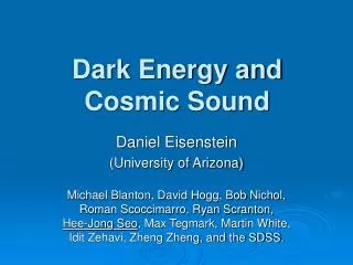
Dark Energy and Cosmic Sound. Daniel Eisenstein (University of Arizona) Michael Blanton, David Hogg, Bob Nichol, Roman Scoccimarro, Ryan Scranton, Hee-Jong Seo , Ed Sirko, David Spergel, Max Tegmark, Martin White, Idit Zehavi , Zheng Zheng, and the SDSS. Dark Energy is Mysterious.

E N D
Dark Energy andCosmic Sound Daniel Eisenstein (University of Arizona) Michael Blanton, David Hogg, Bob Nichol, Roman Scoccimarro, Ryan Scranton, Hee-Jong Seo, Ed Sirko, David Spergel, Max Tegmark, Martin White,Idit Zehavi, Zheng Zheng, and the SDSS.
Dark Energy is Mysterious • Observations suggest that the expansion of the universe is presently accelerating. • Normal matter doesn’t do this! • Requires exotic new physics. • Cosmological constant? • Very low mass field? • Some alteration to gravity? • We have no compelling theory for this! • Need observational measure of the time evolution of the effect.
dr = (c/H)dz dr = DAdq Observer A Quick Distance Primer • The homogeneous metric is described by two quantities: • The size as a function of time,a(t). Equivalent to the Hubble parameter H(z) = d ln(a)/dt. • The spatial curvature, parameterized by Wk. • The distance is then (flat) • H(z) depends on the dark energy density.
Dark Energy is Subtle • Parameterize by equation of state, w = p/r, which controls how the energy density evolves with time. • Measuring w(z) requires exquisite precision. • Varying w assuming perfect CMB: • Fixed Wmh2 • DA(z=1000) • dw/dz is even harder. • Need precise, redundant observational probes! Comparing Cosmologies
Outline • Baryon acoustic oscillations as a standard ruler. • Detection of the acoustic signature in the SDSS Luminous Red Galaxy sample at z=0.35. • Cosmological constraints therefrom. • Large galaxy surveys at higher redshifts. • Future surveys could measure H(z) and DA(z) to few percent from z=0.3 to z=3. • Assess the leverage on dark energy and compare to alternatives.
Acoustic Oscillations in the CMB • Although there are fluctuations on all scales, there is a characteristic angular scale.
Acoustic Oscillations in the CMB WMAP team (Bennett et al. 2003)
Before recombination: Universe is ionized. Photons provide enormous pressure and restoring force. Perturbations oscillate as acoustic waves. After recombination: Universe is neutral. Photons can travel freely past the baryons. Phase of oscillation at trec affects late-time amplitude. Recombination z ~ 1000 ~400,000 years Big Bang Neutral Ionized Today Time Sound Waves in the Early Universe
Sound Waves • Each initial overdensity (in DM & gas) is an overpressure that launches a spherical sound wave. • This wave travels outwards at 57% of the speed of light. • Pressure-providing photons decouple at recombination. CMB travels to us from these spheres. • Sound speed plummets. Wave stalls at a radius of 150 Mpc. • Overdensity in shell (gas) and in the original center (DM) both seed the formation of galaxies. Preferred separation of 150 Mpc.
A Statistical Signal • The Universe is a super-position of these shells. • The shell is weaker than displayed. • Hence, you do not expect to see bullseyes in the galaxy distribution. • Instead, we get a 1% bump in the correlation function.
Remember: This is a tiny ripple on a big background. Response of a point perturbation Based on CMBfast outputs (Seljak & Zaldarriaga). Green’s function view from Bashinsky & Bertschinger 2001.
Acoustic Oscillations in Fourier Space • A crest launches a planar sound wave, which at recombination may or may not be in phase with the next crest. • Get a sequence of constructive and destructive interferences as a function of wavenumber. • Peaks are weak — suppressed by the baryon fraction. • Higher harmonics suffer from Silk damping. Linear regime matter power spectrum
Acoustic Oscillations, Reprise • Divide by zero-baryon reference model. • Acoustic peaks are 10% modulations. • Requires large surveys to detect! Linear regime matter power spectrum
dr = (c/H)dz dr = DAdq Observer A Standard Ruler • The acoustic oscillation scale depends on the sound speed and the propagation time. • These depend on the matter-to-radiation ratio (Wmh2) and the baryon-to-photon ratio (Wbh2). • The CMB anisotropies measure these and fix the oscillation scale. • In a redshift survey, we can measure this along and across the line of sight. • Yields H(z) and DA(z)!
Galaxy Redshift Surveys • Redshift surveys are a popular way to measure the 3-dimensional clustering of matter. • But there are complications from: • Non-linear structure formation • Bias (light ≠ mass) • Redshift distortions • Do these affectthe acousticsignatures? SDSS
Nonlinearities & Bias • Non-linear gravitational collapse erases acoustic oscillations on small scales. However, large scale features are preserved. • Clustering bias and redshift distortions alter the power spectrum, but they don’t create preferred scales at 100h-1 Mpc! • Acoustic peaks expected to survive in the linear regime. z=1 Meiksen & White (1997), Seo & DJE (2005)
Virtues of the Acoustic Peaks • Measuring the acoustic peaks across redshift gives a purely geometrical measurement of cosmological distance. • The acoustic peaks are a manifestation of a preferred scale. • Non-linearity, bias, redshift distortions shouldn’t produce such preferred scales, certainly not at 100 Mpc. • Method should be robust, but in any case the systematic errors will be very different from other schemes. • However, the peaks are weak in amplitude and are only available on large scales (30 Mpc and up). Require huge survey volumes.
Introduction to SDSS LRGs • SDSS uses color to target luminous, early-type galaxies at 0.2<z<0.5. • Fainter than MAIN (r<19.5) • About 15/sq deg • Excellent redshift success rate • The sample is close to mass-limited at z<0.38. Number density ~ 10-4h3 Mpc-3. • Science Goals: • Clustering on largest scales • Galaxy clusters to z~0.5 • Evolution of massive galaxies
Intermediate-scale Correlations Redshift-space Real-space • Subtle luminosity dependence in amplitude. • s8 = 1.80±0.03 up to 2.06±0.06 across samples • r0 = 9.8h-1 up to 11.2h-1 Mpc • Real-space correlation function is not a power-law. Zehavi et al. (2004)
Acoustic series in P(k) becomes a single peak in x(r)! Pure CDM model has no peak. Warning: Correlated Error Bars Large-scale Correlations
Another View CDM with baryons is a good fit: c2= 16.1 with 17 dof.Pure CDM rejected at Dc2= 11.7
A Prediction Confirmed! • Standard inflationary CDM model requires acoustic peaks. • Important confirmation of basic prediction of the model. • This demonstrates that structure grows from z=1000 to z=0 by linear theory. • Survival of narrow feature means no mode coupling.
Equality scale depends on (Wmh2)-1. Wmh2 = 0.12 Wmh2 = 0.13 Wmh2 = 0.14 Acoustic scale depends on (Wmh2)-0.25. Two Scales in Action
Parameter Estimation • Vary Wmh2 and the distance to z = 0.35, the mean redshift of the sample. • Dilate transverse and radial distances together, i.e., treat DA(z) and H(z) similarly. • Hold Wbh2 = 0.024, n = 0.98 fixed (WMAP). • Neglect info from CMB regarding Wmh2, ISW, and angular scale of CMB acoustic peaks. • Use only r>10h-1 Mpc. • Minimize uncertainties from non-linear gravity, redshift distortions, and scale-dependent bias. • Covariance matrix derived from 1200 PTHalos mock catalogs, validated by jack-knife testing.
Pure CDM degeneracy Acoustic scale alone WMAP 1s Cosmological Constraints 2-s 1-s
A Standard Ruler • If the LRG sample were at z=0, then we would measure H0 directly (and hence Wm from Wmh2). • Instead, there are small corrections from w and WK to get to z=0.35. • The uncertainty in Wmh2 makes it better to measure (Wmh2)1/2D. This is independent of H0. • We find Wm = 0.273 ± 0.025 + 0.123(1+w0) + 0.137WK.
Essential Conclusions • SDSS LRG correlation function does show a plausible acoustic peak. • Ratio of D(z=0.35) to D(z=1000) measured to 4%. • This measurement is insensitive to variations in spectral tilt and small-scale modeling. We are measuring the same physical feature at low and high redshift. • Wmh2 from SDSS LRG and from CMB agree. Roughly 10% precision. • This will improve rapidly from better CMB data and from better modeling of LRG sample. • Wm = 0.273 ± 0.025 + 0.123(1+w0) + 0.137WK.
Constant w Models • For a given w and Wmh2, the angular location of the CMB acoustic peaks constrains Wm (or H0), so the model predicts DA(z=0.35). • Good constraint on Wm, less so on w (–0.8±0.2).
L + Curvature • Common distance scale to low and high redshift yields a powerful constraint on spatial curvature:WK = –0.010 ± 0.009 (w = –1)
Power Spectrum • We have also done the analysis in Fourier space with a quadratic estimator for the power spectrum. • The results are highly consistent. • Wm = 0.25, in part due to WMAP-3 vs WMAP-1. • Also FKP analysis in Percival et al. (2006). Tegmark et al. (2006)
Beyond SDSS • By performing large spectroscopic surveys at higher redshifts, we can measure the acoustic oscillation standard ruler across cosmic time. • Higher harmonics are at k~0.2h Mpc-1 (l=30 Mpc) • Measuring 1% bandpowers in the peaks and troughs requires about 1 Gpc3 of survey volume with number density ~10-3 comoving h3 Mpc-3 = ~1 million galaxies! • Discuss survey optimization then examples.
Non-linearities Revisited • Non-linear gravitational collapse and galaxy formation partially erases the acoustic signature. • This limits our ability to centroid the peak and could in principle shift the peak to bias the answer. Meiksen & White (1997), Seo & DJE (2005)
Nonlinearities in x(r) • The acoustic signature is carried by pairs of galaxies separated by 150 Mpc. • Nonlinearities push galaxies around by 3-10 Mpc. Broadens peak, erasing higher harmonics. • Moving the scale requires net infall on 100 h–1 Mpc scales. • This depends on the over-density inside the sphere, which is about J3(r) ~ 1%. • Over- and underdensities cancel, so mean shift is <<1%. • Simulations show no evidencefor any bias at 1% level. Seo & DJE (2005); DJE, Seo, & White, in press
Nonlinearities in P(k) • How does nonlinear power enter? • Shifting P(k)? • Erasing high harmonics? • Shifting the scale? • Acoustic peaks are more robost than one might have thought. • Beat frequency difference between peaks and troughs of higher harmonics still refers to very large scale. Seo & DJE (2005)
Where Does Displacement Come From? • Importantly, most of the displacement is due to bulk flows. • Non-linear infall into clusters "saturates". Zel'dovich approx. actually overshoots. • Bulk flows in CDM are created on large scales. • Looking at pairwise motion cuts the very large scales. • The scales generating the displacements are exactly the ones we're measuring for the acoustic oscillations. DJE, Seo, Sirko, & Spergel, in press
Fixing the Nonlinearities • Because the nonlinear degradation is dominated by bulk flows, we can undo the effect. • Map of galaxies tells us where the mass is that sources the gravitational forces that create the bulk flows. • Can run this backwards. • Restore the statistic precision available per unit volume! DJE, Seo, Sirko, & Spergel, in press
Cosmic Variance Limits Errors on D(z) in Dz=0.1 bins. Slices add in quadrature. Black: Linear theory Blue: Non-linear theory Red: Reconstruction by 50% (reasonably easy) Seo & DJE, submitted
Cosmic Variance Limits Errors on H(z) in Dz=0.1 bins. Slices add in quadrature. Black: Linear theory Blue: Non-linear theory Red: Reconstruction by 50% (reasonably easy) Seo & DJE, submitted
Seeing Sound in the Lyman a Forest • The Lya forest tracks the large-scale density field as well, so a grid of sightlines should show the acoustic peak. • This may be a cheaper way to measure the acoustic scale at z>2. • Bonus: the sampling is better in the radial direction, so favors H(z). • Require only modest resolution (R=250) and low S/N. UV coverage is a big plus. Green line is S/N=2 Å–1at g=22.5 White (2004); McDonald & DJE (2006)
Chasing Sound Across Redshift Distance Errors versus Redshift
APO-LSS • New program for the SDSS telescope for the period 2008–2014. 10,000 deg2 of new spectroscopy from SDSS imaging. • 1.5 million LRGs to z=0.8, including 4x more density at z<0.5. • 7-fold improvement on large-scale structure data from entire SDSS survey, measure the distance scale to better than 1%. • Lya forest from grid of 100,000 z>2.2 quasars. • Mild upgrades to the spectrographs to reach 1000 fibers per shot and more UV coverage. • Other aspects of the program include stellar spectroscopic survey for galactic structure and a multi-fiber radial-velocity planet search. • Collaboration now forming.
New Surveys • WiggleZ: Survey of z~0.8 emission line galaxies at AAT with new AAOmega upgrade. • FMOS: z~1.5 Subaru survey with IR spectroscopy for Ha. • HETDeX: Lya emission galaxy survey at 1.8<z<3.8 with new IFU on HET. • New WFMOS spectrograph for Gemini/Subaru could do major z~1 and z~2.5 surveys in ~100 nights each. • Well ranked in Aspen second-generation instruments plan. Currently entering a competitive design study. • 1.5 degree diameter FOV, 4000-5000 fibers, using Echidna technology, feeding multiple bench spectrographs. • Also high-res for Galactic studies.
Concept proposed for the Joint Dark Energy Mission (JDEM). • 3/4-sky survey of 1<z<2 from a small space telescope, using slitless IR spectroscopy of the Ha line. SNe Ia to z~1.4. • 100 million redshifts; 20 times more effective volume than previous ground-based surveys. • Designed for maximum synergy with ground-based dark energy programs.
Breaking the w-Curvature Degeneracy • To prove w ≠ –1, we should exclude the possibility of a small spatial curvature. • SNe alone, even with space, do not do this well. • SNe plus acoustic oscillations do very well, because the acoustic oscillations connect the distance scale to z=1000.
Constraining w(z) • Data sets: • CMB (Planck) • SNe: 1% in D from z=0.05 to z=0.95 in Dz=0.1 bins. • Current SDSS (red) • APO-LSS (black) • +WFMOS (blue) • +ADEPT (magenta). • w(z) as cubic polynomial, including spatial curvature. • BAO can add w(z) measurement at z>1. 95% contours Dark Energy Constraints around LCDM
Opening Discovery Spaces • With CMB and galaxy surveys, we can study dark energy out to z=1000. • SNe should do better at pinning down D(z) at z<1. But acoustic method opens up z>1 and H(z) to find the unexpected. • Weak lensing, clusters also focus on z<1. These depend on growth of structure. We would like both a growth and a kinematic probe to look for changes in gravity.
Photometric Redshifts? • Can we do this without spectroscopy? • Measuring H(z) requires detection of acoustic oscillation scale along the line of sight. • Need ~10 Mpc accuracy. sz~0.003(1+z). • But measuring DA(z) from transverse clustering requires only 4% in 1+z. • Need ~half-sky survey to match 1000 sq. deg. of spectra. • Less robust, but likely feasible. 4% photo-z’s don’t smearthe acoustic oscillations.