Download
1 / 52
530 likes | 647 Vues
Chapter 6 RESISTANCE THERMOMETRY. 6.1 Principles

E N D
Chapter 6 RESISTANCE THERMOMETRY
6.1 Principles A resistance the thermometer is a temperature-measuring instrument consisting of a sensor , an electrical circuit element whose resistance varies with temperature; a framework on which to support the sensor;a sheath by which the sensor is protected;and wires by which the sensor is connected to a measuring instrument(usually a bridge),which is used to indicate the effect of variations in the sensor resistance.
Sir Humphry Davy had noted as early as 1821 that the conductivity of various metals was always lower in some inverse ratio as the temperature was higher. Sir William Siemens, in 1871 first outlined the method of temperature measurement by means of a platinum resistance thermometer. It was not until 1887,however,that precision resistance thermometry as we know it today began. This was when Hugh Callendar’s published his famous paper on resistance thermometers [1].Callendar’s equation describing the variation in platinum resistance with temperature is still pertinent; it is now used in part to define temperature on the IPTS(see Chapter 4)from the ice point to the antimony point.
Resistance thermometers provide absolute temperatures in the sense that no reference junctions are involved, and no special extension wires are needed to connect the sensor with the measuring instrument. The three s that characterize resistance the thermometers are simplicity of circuits sensitivity of measurements, and stability of sensors.
6.2 Sensors The sensors [2],[3] can be divided conveniently into two basic groups: resistance temperature detectors (RTDs) and thermistors RTDs are electrical circuit elements formed of solid conductors(usually in wire form) that are characterized by a positive coefficient of resistivity. It is interesting to note in this regard that there is a direct relation between the temperature coefficient of resistivity of metals and the coefficient of expansion of gases . The RTDs of general usage are of platinum, nickel and copper.
Platinum sensors Platinum being a noble metal , is used exclusively for precision resistance thermometers .Platinum is stable (i.e. it is relatively indifferent to its environment, it resists corrosion and chemical attack, and it is not readily oxidized ), is easily workable (i.e., it can be drawn into fine wires), has a high melting point (i.e. it shows little volatilization below 1000℃), and can be obtained to a high degree of purity (i.e. it has reproducible electrical and chemical characteristics). All this is evidenced by a simple and stable resistance-temperatures (R-T) relationship that characterizes the platinum sensor over a wide range of temperatures.
These desirable and necessary features. however, do not came without effort. Platinum is actually extremely sensitive to minute contaminating impurities and to strains (to avoid the strain gage effect whereby extraneous changes in resistance occur ), and the thermometer must be manufactured in a manner that ensures freedom from contaminants. These two effects are guarded against by elaborate precautions.
Since the time of Callendar, the sensors have been constructed by forming a coil of very pure platinum wire around two mica strips that are joined to form a cross , Meyers [4],at the National Bureau of Standards , first wound the wire in a fine helical coil around a steel wire mandrel, and then wound this coil helically around a mica cross framework ( see Figure 6.1) .
Such procedures leave the wire relatively free from mechanical constraints as the wire experience differential thermal expansions . The sensor is also annealed to relieve winding strains . The diameter of the platinum wire is on the order of 0.1 mm , and it takes a length of about 2m to yield a satisfactory 25.5Ω resistance at the ice point. The resulting precision platinum sensors are usually about 1 in. long。
The sensors are then assembled in a protecting sheath ( usually a tube of pyrex or quartz ) about 18 in. long with four gold wires joining the sensor at the bottom of the tube to four copper connecting wires outside the tube . The tube assembly is evacuated and filled with dry air at about one-half atmosphere and hermetically sealed to exclude contaminants . Mica disks separate the internal connecting wires and also serve to break up any convection currents in the tube [ 5 ] .
Construction is such that δ(the characteristic coefficient of the particular thermometer as determined at the zinc point) is between 1.488 and 1.498 . The purity of the platinum wires is assured by testing at the ice and steam point, where R100/R0 must be greater than 1.3925 , where the higher this value , the greater the purity of the platinum . The reasons for the temperature limitation of present-day platinum res stance thermometers are threefold: 1. The pyrex tube yields to stresses above 1000℉. 2. The water of crystallization in the mica insulators may distort the mica above 1000 ℉.
3. The platinum wire may become, sensibly thinner ( by evaporation )at the higher temperatures , and this would cause an increase in resistance . The National Bureau of Standards hopes to extend the range of the platinum resistance thermometer standard from the antimony to the gold point , in accord with proposals of H.Moser[6] of Germany , by use of special sheaths and special insulators . Several papers describing studies on long-term stability and performance of gold point resistance- thermometer have been published [7] ,[8] . Their conclusion is that high temperature resistance thermometers can lead to a better practical temperature scale up to the gold point just as prognosticated in section 4.4.2 .
Meantime , good precision platinum resistance thermometers are commercially available with NBS certificates up to 1000 ℉, so that construction details need not be discussed further here . Nickel and Copper Sensors These are much cheaper than the platinum sensors and are useful in many special applications. Nickel is appreciably nonlinear , however , and has an upper temperature limit of about 600 ℉ . Copper is quite linear , but is limited to about 250 ℉ , and has such a low resistance .that very accurate measurements are required. All in all, the platinum RTDs continue to dominate the field in present resistance thermometry.
Thermistors Temperature-sensitive resistor materials (such as metallic oxides) have been known to science for some time. However ,the chief stumbling block to the widespread use of these materials was their lack of electrical and chemical stability. In 1946, Becker, Green, and Pearson , at the Bell Laboratories , reported [9] on success in producing metallic oxides that had high negative coefficients of resistivity and exhibited the stable characteristics necessary for manufacturing to reproducible, specifications. Thus thermistors ( a contraction for "thermally sensitive resistors") are electrical circuit elements formed of solid semi- conducting materials that are characterized by a high negative co- efficient of resistivity .
At any fixed temperature , a thermistor acts exactly as any ohmic conductor . If its temperature is permitted to change , however , either as a result of a change in ambient conditions or because of a dissipation of electrical power in it , the resistance of the thermistor is a definite , reproducible function of its temperature . Typical thermistor resistance variations are function of its temperature. Typical thermistor resistance variation are from 50,000Ω at 100℉ to 200Ω at 500℉. Their characteristic temperature-resistance relationship can approximated by a power function of the form R=aeb/T (6.1)
where R is the thermistor resistance at its absolute ambient temperature T , and a and b are constants for the particular thermistor under consideration , with typical values of 0.06 and 8000 , respectively. Note that the logarithm of R plots as a straight line of intercept log a and slope b, when charted versus (l/T). Their use for temperature measurement is based on the direct or indirect determination of the resistance of a thermistor immersed in the environment whose temperature is to be measured . Because we are dealing with an ohmic circuit ,ordinary copper wires suffice throughout the thermistor circuit; thus special extension wires,reference junctions , and bothersome thermal emfs are avoided .
Contrary to common belief , thermistor are quite stable when they are properly aged before use ( less than 0.1% drift in resistance during periods of months). Thermistors exhibit great temperature sensitivity (up to ten times the sensitivity of the usual base-metal thermocouples), whereas thermistor response can be in the order of milliseconds . The practical range for which the thermistor are useful is from the ice point to about 6000 ℉[10]. Routine temperature measurements to 0.1oF are not unusual if the current through a thermistor is limited to a value that does not increase the thermistor temperature (by I2R heating) above ambient by an amount greater than that consistent with the measuring accuracy required .
6.3 Circuits and Bridges The conventional Wheatstone bridge circuit( Figure6 .2a) is not very satisfactory for platinum resistance thermometry because (a) the slide-wire contact resistance is a variable depending on the condition of the slide ; (b) the resistance of the extension wires to the sensor is a variable depending on the temperature gradient along them ; (c) the supply current itself causes variable self-heating depending on the resistance of the sensor [11] . The three extension-wire Callendar - Griffiths bridge circuit, Figure 6.2b, while alleviating some of the faults of the Wheatstone bridge, still is not entirely satisfactory .
The four-extension-wire Mueller bridge circuit , Figure 6.2c, is almost always used to determine the platinum sensor resistance . Most of the important measuring resistors are protected from ambient temperature changes by incorporating them in a thermostatically controlled constant-temperature chamber . The range of resistance for which these bridge are intended is from 0.0 to 422.llllΩ. The temperature rise caused by the bridge current must be kept small so that no reduction in the current produces an observable change in the indication or resistance . In direct opposition to this requirement of low self-heating current is the fact that for maximum bridge sensitivity the bridge current should be as large as possible .
Since the time of his 1939 paper [12] , Mueller has designed a new bridge for precision resistance thermometry. H. F. Stimson, at the NBS, gave a brief description of this bridge somewhat as follows [13]. The intention of the design was to make measurements possible within an
Figure 6.2 (a)Conventional Wheatstone bridge circuit. When G is zeroed by moving Rslide , IsensorRsensor=IslideRslide and IsensorRA=IslideRB .Dividing one by the other , Rsensor=(RA/RB) Rslide ; therefore Rsensoris easily determined by fixed ratio (RA/RB) and the variable Rslide which is obtained from the calibrated scale . (b) The Callendar-Griffiths bridge circuit ,in which slide-wire contact has no effect of extension-lead resistance variation is reduced , and the effect of self-heating of the sensor is reduced if RA= Rsensor . (c) The Mueller bridge circuit . With the switch in one position (as shown), R1+RT=Rsensor+ RC.
With the switch in the other position, extension leads C and T and CD and T are interchanged. respectively ,and RD2+RC = Rsensor+RT . then, by addition, Rsensor=(RD1+RD2)/2 and the effects of the extension leads have been eliminated. Uncertainty not exceeding 2 or 3μΩ . This bridge has a seventh decade that makes one step in the last decade the equivalent of 10μΩ. One uncertainty that was recognized was that of the contact resistance in the dial switches of the decades . Experience shows that with care this uncertainty can be kept down to the order of 0.0001Ω .
In Mueller's design , the ends of the equal-resistance ratio arms are at the dial-switch contacts on the lΩ and the 10Ω decades . He has made the resistances of the ratio arm 3000Ω; thus the uncertainty of contact resistance , 0.0001Ω, produces an uncertainty of only one part in 30, 000,000 . With 30Ω,for example , in each of the other arms of the bridge , these two ratio-arm contacts should produce an uncertainty of resistance measurement of 1.41μΩ . The 10Ω decade has mercury contacts and the commutator switch has large mercury contacts . one new feature in the commutator switch is the addition of an extra pair of mercury-contact links that serve to reverse the ratio coils simultaneously with the thermometer leads .
This feature automatically makes the combined error of the normal and reverse readings only one in a million , for example, when the ratio arms are unequal by as much as one part in a thousand , and thus almost eliminates any error from lack of balance in the ratio arms . It does not eliminate any systematic error in the contact resistance at the end of the ratio arms on the decades , however , because the mercury reversing switch must be in the arms . The commutators on these bridges are made so as to open the battery circuit before breaking contacts in the resistance leads to the thermometer . This makes it possible to lift the commutator , rotate it , and set it down in the reverse position in less than a second and thus not disturb the galvanometer or the steady heating of the resistor by a very significant amount .
In balancing the bridge , snap switches are used to reverse the current so the heating is interrupted only a small fraction of a second . This practice of reversing the current has proved very valuable . It not only keeps the current flowing almost continuously in the resistor but also gives double the signal of the bridge unbalances . Basic thermistor circuits are given in Figure 6 .3a and b. one is the familiar Wheatstone bridge , and the other is a simple series circuit that is quite effective in determining thermistor temperature as a function of the emf drop across a fixed resistor .
6 .4 Equation and Solutions In Chapter 4 the Callendar interpolating equation for the platinum resistance thermometer , which was used in part to define temperature on the IPTS between the ice and antimony points , was given by(4.1) as (6.2) Similarly , between the oxygen and ice points , the Callendar - VanDusen equation was given by (4 .2). The point here is that it is one thing to measure a resistance precisely ( no mean feat in itself , as indicated in Section6.3) and quite another to convert the measurement readily to a temperature .
Hand calculations , involving quadratics and cubics , are practical if only a few conversions are required . Eggenberger [ 14 ] has Presented a solution to (6 .2) , based in part on tables and in part on graphs . With the advent of the computer , machine solution make resistance-to-temperature conversions routine , precise ,and nearly instantaneous[15].Note that (6 .2) , for example , also can be expressed as (6.3) Solving the quadratic yields (6.4)
where Equation 6 .3 can be solved readily by hand , whereas(6.4) may be more amenable to machine solution . However , (6.4) may be manipulated still further to obtain Eggenberger’s tabular-graphical solution ; that is , to avoid solution of (6 .4) for each measurement , the temperature also can be expressed as
(6.5) where t = the empirical temperature corresponding to the total resistance measurement ; tl =that part of the temperature measurement corresponding to the integral part of the resistance measurement ; Δt = the approximate part of the temperature measurement corresponding to the decimal part of the resistance measurement (the approximation is that the slope⊿t/⊿R is 10℃/Ω) ; correction = the adjustment necessary to account for the approximation of a constant temperature-resistance slope .
Equation 6.5 is synthesized as follows . First, the resistance (Rt) of ( 6 .4 ) is expressed in parts . Thus (6.6) where Rirepresents the integral part of the resistance, and △R the decimal part . The temperature corresponding to the integral part of the resistance is then (6.7) This expression can be tabulated for the individual resistance thermometer ( e. g ., see Table 6.l ). The approximate temperature, including the integral part of the resistance plus the approximate effect of the decimal part of the resistance is
(6.8) where S = ( C-Ri ) , and the slope , △t/△R , is assumed to be 10℃/Ω( or18℉/Ω). The complete expression for the temperature is then (6.9) Expressed as a correction ,(6.9) yields (6.10) This correction can be plotted for the individual resistance thermometer (e.g., see Figurc 6 . 4 ) .
Table 6.1 Typical Platinum Resistance Thermometer Chart ( absolute ohms versus degrees Fahrenheit )
Example 1. A platinum resistance thermometer having the constants R0=25.517Ω, R100/ R0=1.392719, and δ=1.493 , indicate Ri=28.5547Ω. What is the corresponding Callendar temperature on the Fahrenheit scale ? A . By hand calculation of ( 6.3)
B . By machine calculation of (6.4 ) t=30℃=86℉(see table 6.2) C . By Eggenberger’s method of ( 6 .5) R1=28Ω,t1=76.106℉(see Table 6.1) ΔR=0.5547Ω,Δt=℉9.98℉ Correction= -0.084(see Figure 6.4) Summing: t=76.106+9.985-0.084=86.007℉ 6 .5 The Calendar Coefficients In this section , we consider a practical method for determining the required resistance thermometer interpolating equations [16] , [17] . According to (4.11), namely,
T68=t’+Δt (6.12) We are assured that the Callendar temperature ,t', as defined by (6.2), is still very important in determining T68 . IPTS-68 calls for the platinum resistance thermometer to be calibrated at the triple point of water (0.01℃), the steam point (100℃),and the zinc point(419.58℃). However, it is common practice to use the tin point(231.9681℃) in place of the steam point. This complicates the computation of the Callendar coefficients in that R100 may not be available experimentally. Hence , to evaluate the Callendar interpolation equation used to obtain t68 one must determine δ and R100analytically . A detailed description for doing this is given next.
Example 3. A certain resistance thermometer exhibits the following resistance at the fixed point of interest: Resisitance temperature R,Ω Fixed point t68℃ 25.56600 Triple 0.01 48.39142 Tin 231.9681 65.67700 Zinc 419.58 These resistance represent the means of many experimental determinations ,
DETERMINATION of CALLENDAR TEMPERATURE of TIN . Although the Callendar temperatures of the triple and zinc points are identical with t68s , since △tS at these points are zero ( see equation 4 .12) , this cannot be said of the tin point . The temperature correction at the tin point is △tSN = 0 . 038937℃ as determined by a short iterative procedure . First, t is assumed equal to t68 and △t is calculated from (4 .12). Then , t is adjusted for this △t according to (6 .12) . The process is repeated until t does not change by more than some acceptable value , say 1 in the fifth decimal place . For the △t so determined ,△tSN = 231.92916℃ .
DETERMINATION OF CALLENDAR COEFFICIENTS b AND c . The Callendar equation can be written in the entirely equivalent form Rt=R0+bt+ct2 (6.13) where the two unknown coefficients can be determined from the algebraic relations where tSN= Callendar temperature at the tin point tZN= Carllendar temperature at the zinc point RSN =Measured resistance at the tin point RZN =Measured resistance at the zinc point
R0 =Measured resistance at the ice point ( this should be about 0.001Ω less than the triple point resistance ). For the value given in this example , b = 1.019045×10⁻¹c=- 1.502488 ×10⁻⁵ DETERMINATION OF R100. Although R100 is no longer a measured quantity , it can be determined readily from (6.13) written as R100=R0+b(102)+c(104) (6.16) For the values given , R100=35.6052Ω and R100//R=1.3927323 .
DETERMINATION OF δ As indicated earlier ,the characteristic constant of the thermometer can be determined from any fixed point data other than the ice and steam points .For example : where pt=100 (Rt-R0)/(R100-R0) and pt is known as the platinum temperature . For the values given ,δ=1.496472 , and ptSN= 227.35022℃ and ptZN=399.51390℃ . Note that the platinum temperatures and the resistances measured at the fixed points are independent of the temperature scale being used .
GENERAL OBSERVATIONS . (l) Since the IPTS-68 △t is zero at the ice , steam , zinc , and antimony points , it follows that the R –t68 points representing these baths are all on the 68-Callendar parabola . (2) It further follows that the tin and sulfur points are not . △tsNhas already been given in this example , By the same method , △tsu=-0.012174(See Figure 6.5). (3) Given the Callendar constants , b and c . and the 68-Callendar temperatures at the sulfur and antimony points ,the corresponding resistances can be determined from (6.13) as R SU = 67.90940Ωand RSD= 83.8628Ω.
4. A contain resistance thermometer yields the following resistance at the fixed points of interest: • Resistance temperature • R,Ω Fixed point t68℃ • 6.2268 oxygen -182.962 • 25.5500 ice 0 • 35.5808 steam 100 • 65.67700 Zinc 419.58 RESISTANCE THERMOMITER COEFFICIENTS . Platinum temperature at the zinc point : ptZN=100(RZN-R0)/(R100-R0)=4007.46/10.0308=399.5158℃
Fundamental coefficient : α=(R100-R0)/(100R0)=10.0308/2555.00=0.0039259591 Callendar constant : VanDusen Constant :
where tQX= Callendar - VanDusen temperature at the oxygen point ROX =measured resistance at the oxygen point . Measured resistance ratios : By equation 4.10 and Table 4.6 :
Also , by Table4 .6 , the interpolating polynomial for determining deviations in Range l , Part 4 is: By simultaneous solution at the oxygen and steam points , the constants , A4and C4 , are determined to be : With this information about this resistance thermometer available , we can ask for example : If the measured resistance ratio is W4=0.5 , what is t68?