Download
1 / 67
670 likes | 969 Vues
Lecture 3 Radiative and Convective Energy Transport. Mechanisms of Energy Transport Radiative Transfer Equation Grey Atmospheres Convective Energy Transport Mixing Length Theory. The Sun. I. Energy Transport.

E N D
Lecture 3Radiative and Convective Energy Transport • Mechanisms of Energy Transport • Radiative Transfer Equation • Grey Atmospheres • Convective Energy Transport • Mixing Length Theory
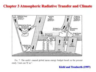
I. Energy Transport In the absence of sinks and sources of energy in the stellar atmosphere, all the energy produced in the stellar interior is transported through the atmosphere into outer space. At any radius, r, in the atmosphere: 4pr2F(r) = constant = L Such an energy transport is sustained by the temperature gradient. The steepness of this gradient is in turn dependent on the effectiveness of the energy transport through the different layers
I. Mechanisms of Energy Transport • Radiation Frad (most important) • Convection: Fconv (important in cool stars like the Sun) • Heat production: e.g. in the transition between the solar chromosphere and corona • Radial flow of matter: coronae and stellar winds • Sound waves: chromosphere and coronae Since we are dealing with the photosphere we are mostly concerned with 1) and 2)
s ∫ tn= knr dx 0 dtn= knrds I. Interaction between photons and matter Absorption of radiation: In In +dIn s kn : mass absorption coefficient [kn] = cm2 gm–1 dIn = –knr In dx Optical depth (dimensionless) Convention: tn = 0 at the outer edge of the atmosphere, increasing inwards
In e Optical Depth In(s) In0 The intensity decreases exponentially with path length → dIn = –In dt = In(s) In0e–tn If t = 1 → In = ≈ 0.37 In0 We can see through the atmosphere until tn~1 Optically thick: t > 1 Optically thin: t < 1
Optical depth, t, of ring material small Optical depth, t, of ring material larger Optical path length larger and you see nebular material as ring Optical path length small and you see central star and little nebular material Optical path length roughly the same one sees disk and no central star
s Optical Depth The quantity t = 1 has a geometrical interpretation in terms of the mean free path of a photon: t = 1 = ∫ krds = krs s ≈ (kr)–1 s is the distance a photon will travel before it gets absorbed. In the stellar atmosphere the abosrbed will get re-emitted and thus will undergo a „random walk“. For a random walk the distance traveled in 1-D is s√N where N is the number of encounters. In 3-D the number of steps to go a distance R is 3R2/s2. At half the solar radius kr ≈ 2.5 thus s ≈ 0.4cm so it takes ≈ 30.000 years for a photon do diffuse outward from the core of the sun.
Emission of Radiation In + dIn In dx jn dIn = jnr In dx jnis the emission coefficient/unit mass [ ] = erg/(s rad2 Hz gm) jn comes from real emission (photon created) or from scattering of photons into the direction considered.
dIn = –In +jn/kn = –In + Sn dtn II. The Radiative Transfer Equation Consider radiation traveling in a direction s. The change in the specific intensity, In, over an increment of the path length, ds, is just the sum of the losses (kn) and the gains (jn) of photons: dIn = –knrIn +jnr In ds Dividing by knrds which is just dtn
dIn = fbebtn + ebtn dtn df df df = bIn+ ebtn dtn dtn dtn bIn+ ebtn = –In + Sn The Radiative Transfer Equation tn appears alone in the previous equation therefore try solutions of the form In(tn) = febtn. Differentiating this function: Substituting into the radiative transfer equation:
df dtn tn f = ∫ Snetndtn + c0 tn In(tn) = febtn 0 =e–tn∫Sn(tn)etn dtn+ c0e–tn 0 The Radiative Transfer Equation The first two terms on each side are equal if we set b = –1 and equating the second term: e–tn = Sn t is a dummy variable or Set tn = 0 → c0 = In(0)
tn In(tn) =∫Sn(tn)e–(tn–tn) + In(0)e–tn 0 tn–tn In(0)→ tn tn=0 tn At point tn the original intensity, In(0) suffers an exponential extinction of e–tn The intensity generated at tn, Sn(tn) undergoes an extinction of e–(tn–tn) before being summed at point tn. bringing e–tn inside the integral:
tn In(tn) =∫Sn(tn)e–(tn–tn) + In(0)e–tn 0 This equation is the basic intergral form of the radiative transfer equation. To perform the integration, Sn(tn), must be a known function. In some situations this is a complicated function, other times it is simple. In the case of thermodynamic equilibrium (LTE), Sn(T) = Bn(T), the Planck function. Knowing T as a function of x or tn amounts to a solution of the transfer equation.
dz rdq dr dIn ∂In dr ∂In dq = + dz ∂z dz ∂q dz Radiative Transfer Equation for Spherical Geometry After all, stars are spheres! z To observer dIn –In + Sn = knrdz q r y x
Radiative Transfer Equation for Spherical Geometry Assume In has no f dependence and dr = cos q dz r dq = –sin q cosq ∂In sinq ∂In – = –In + Sn knrdr ∂q knrr ∂r This form of the equation is used in stellar interiors and the calculation of very thick stellar atmospheres such as supergiants. In many stars (sun) the photosphere is thin thus we can use the plane parallel approximation
dIn = –In + Sn cosq knrdr dIn cosq = In – Sn dtn Plane Parallel Approximation To observer q ds The increment of path length along the line of sight is ds = dx sec q To center of star q does not depend on z so there is no second term Custom to adopt a new depth variable x defined by dx = –dr. Writing dtn for knrdx:
Therefore the radiative transfer equation becomes: tn In(tn) =–∫Sn(tn)e–(tn–tn)sec q sec q dtn c The integration limit c replaces In(0) integration constant because the boundary conditions are different for radiation going in (q > 90o) and coming out (q < 90o). The optical depth is measured along x and not along the line of sight which is at some angle q. Need to replace tn by –tnsec q. The negative sign arises from choosing dx = –dr In the first case we start at the boundary where tn=0 and work inwards. So when In = Inin, c=0. In the second case we consider radiation at the depth tnand deeper until no more radiation can be seen coming out. When In=Inout, c=∞
∞ = ∫Sne–(tn–tn)sec q sec q dtn tn tn –∫Sne–(tn–tn)sec q sec q dtn 0 Therefore the full intensity at the position tn on the line of sight through the photosphere is: In(tn) = Inout(tn) + Inin(tn) = Note that one must require that Sne–tn goes to zero as tn goes to infinity. Stars obviously can do this!
An important case of this equation occurs at the stellar surface: Inin(0) = 0 ∞ Inout(0) = ∫Sn(tn)e–tnsec q sec q dtn 0 Assumption: Ignore radiation from the rest of the universe (other stars, galaxies, etc.) This is what you need to compute a spectrum. For the sun which is resolved, intensity measurements can be made as a function of q. For stars we must integrate In over the disk since we observe the flux.
p ∫ Incos q sin q dq Fn = 2p p/2 p 0 ∫ ∫ 2p = 2p Inoutcos q sin q dq + Inincos q sin q dq ∫ Incos q dw Fn = 0 p/2 The Flux Integral Assuming no azimuthal (f) dependence
The Flux Integral Using previous definitions of Inin and Inout p/2 ∞ ∫ ∫ Sne–(tn–tn)sec q sin q dtn dq Fn = 2p 0 tn tn p ∫ ∫ Sne–(tn–tn)sec q sin q dtn dq – 2p p/2 0
p/2 p/2 ∞ ∫ ∫ ∫ Fn = 2p Sn e–(tn–tn)sec q sin q dtn dq 0 0 tn tn p ∫ ∫ – 2p Sn e–(tn–tn)sec q sin q dtn dq ∞ 0 p/2 e–xw ∫ dw e–(tn–tn)sec q sin q dtn dq = w2 1 The Flux Integral If Sn is isotropic Let w = sec q and x = tn– tn
∞ ∫ tn tn ∫ Fn(tn)= 2p – 2p Sn E2(tn– tn)dtn Sn E2(tn– tn)dtn 0 ∞ e–xw ∫ dw wn 1 The Flux Integral Exponential Integrals En(x) = In the second integral w = –sec q and x = tn – tn . The limit as q goes from p/2 to p is approached with negative values of cos q so w goes to ∞ not –∞
∞ ∫ 0 The Flux Integral The theoretical spectrum is Fn at tn = 0: Fn is defined per unit area Fn(0)= 2p Sn(tn)E2(tn)dtn In deriving this it was assumed that Sn is isotropic. It most instances this is a reasonable assumption. However, in stars there are Doppler shifts due to photospheric velocities, stellar rotation, etc. Isotropy no longer holds so you need to do an explicit disk integration over the stellar surface, i.e. treat Fn locally and add up all contributions.
tn ∫ Jn(tn)= 1/2 + 1/2 Sn E1(tn– tn)dtn Sn E1(tn– tn)dtn 0 ∞ ∞ ∫ ∫ tn tn tn ∫ Kn(tn)= 1/2 + 1/2 Sn E3(tn– tn)dtn Sn E3(tn– tn)dtn 0 The Mean Intensity and K Integrals
∞ ∞ dEn 1 d e–xw ∫ ∫ e–xw dw dw = = – wn dx dx wn–1 ∞ 1 e–xw 1 ∫ dw wn dEn = –En–1 1 dx The Exponential Integrals Exponential Integrals En(x) = ∞ dw ∫ 1 En(0) = = wn 1–n 1
The Exponential Integrals Recurrence formula En+1(x) = e–x –xEn(x)
n(n+1) x2 1 ≈ xex The Exponential Integrals For computer calculations: From Abramowitz and Stegun (1964) E1(x) = e–x –xEn(x) E1(x) = –lnx – 0.57721566 + 0.99999193x – 0.24991055x2 + 0.05519968 x3 – 0.00976004x4 + 0.00107857x5 for x ≤ 1 x4 + a3x3 + a2x2 + a1x + a0 1 x >1 E1(x) = xex x4 + b3x3 + b2x2 + b1x + b0 a3 = 8.5733287401 b3= 9.5733223454 Assymptotic Limit: b2= 25.6329561486 a2= 18.0590169730 1 [ n … [ 1 – + – En(x) = a1= 8.6347608925 b1= 21.0996530827 xex x b0= 3.9584969228 a0= 0.2677737343 Polynomials fit E1 to an error less than 2 x 10⁻⁷
Radiative Equilibrium • Radiative equilibrium is an expression of conservation of energy • In computing theoretical models it must be enforced • Conservation of energy applies to the flow of energy through the atmosphere. If there are no sources or sinks of energy in the atmosphere the energy generated in the core flows to the outer boundary • No sources or sinks in the atmosphere implies that the divergence of the flux is zero everywhere in the photosphere. In plane parallel geometry: d F(x) = 0 or F(x) = F0 A constant dx ∞ F(x) = ∫F0 (tn)dn =F0 for flux carried by radiation 0
∞ ∫ tn ∞ ∫ 0 Radiative Equilibrium tn [ F0 ∫ [ dn = Sn E2(tn– tn)dtn Sn E2(tn– tn)dtn – 2p 0 This is Milne‘s second equation It says that in the case of radiative equilibrium the solution of the radiative transfer equation is found when Sn is known that satisfies this equation.
dIn cosq = knrIn – knrSn dx ∫ ∫ ∫ dFn dx Radiative Equilibrium Other two radiative equilibrium conditions come from the transfer equation : Integrate over solid angle d = knr In dw – knr Sn dw Incos q dw dx Substitue the definitions of flux and mean intensity in the first and second integrals = 4pknrJn – 4pknrSn
∞ ∞ ∞ ∞ ∞ ∫ ∫ ∫ ∫ ∫ 0 0 0 0 0 Radiative Equilibrium Integrating over frequency d Fn dn = 4pr knJn dn – 4pr knSn dn dx But in radiative equilibrium the left side is zero! knSn dn knJn dn = Note: the value of the flux constant does not appear
tn ∫ Jn(tn)= ½ +½ Sn E1(tn– tn)dtn Sn E1(tn– tn)dtn 0 ∞ ∞ ∞ ∫ ∫ ∫ tn tn 0 tn ∫ 0 Radiative Equilibrium Using expression for Jn [ [ kn ½ Sn E1(tn– tn)dtn + ½ dn = 0 Sn E1(tn– tn)dtn First Milne equation
F0 ∞ ∞ ∞ ∫ ∫ 4p ∫ ∫ ∫ d 0 tn 0 dtn 4p [ tn [ ½ Sn E3(tn– tn)dtn + ½ dn SnE3(tn– tn)dtn = ∫ 0 Radiative Equilibrium If you multiply radiative equation by cos q you get the K-integral dIn dw cos2q dw knrIncos q– knrSn cos q = dx 2nd moment 1st moment dKn F0 And integrate over frequency dn = dtn Third Milne Equation
Radiative Equilibrium The Milne equations are not independent. Sn that is a solution for one is a solution for all three The flux constant F0 is often expressed in terms of an effective temperature, F0 = sT4. The effective temperature is a fundamental parameter characterizing the model. In the theory of stellar atmospheres much of the technical effort goes into iterative schemes using Milne‘s equations of radiative equilibrium to find the source function, Sn(tn)
∞ ∞ ∞ ∞ ∞ F = ∫Fndn K = ∫Kndn S = ∫Sndn J = ∫Jndn I = ∫Indn 0 0 0 0 0 dI cosq = –I + S dt III. The Grey Atmosphere The simplest solution to the radiative transfer equation is to assume that kn is independent of frequency, hence the name „grey“. It occupies an „historic“ place and is the starting point in many iterative calculations. Electron scattering is the only opacity source relevant to stellar atmospheres that is independent of frequency. Integrate the basic transfer equation over frequency and denote: Where dt = krdx, the „grey“ absorption coefficient
dK F0 = dt 4p The Eddington approximation, hemispherically isotropic outward and inward specific intensity: Iout(t) for 0 ≤ q ≤ p/2 I(t) = Iin(t) for p/2 ≤ q ≤ p The Grey Atmosphere This grey case simplifies the radiative equilibrium and Milne‘s equations: F(x) = F0 J = S
p p/2 ∫ ∫ J = Idw = + Iout Iin sin q dq sin q dq 0 p/2 1 ∫ = Iout (t)+ Iin(t) 4p 1 1 1 1 2 6 2 2 F(t) = p Iout (t)–Iin(t) K(t) = Iout (t)+ Iin(t) The Grey Atmosphere But since the mean intensity equals the source function in this case S(t) = J(t) = 3K(t)
F0 F0 K(t) = + t 6p 4p dK F0 = dt 4p 3F0 (t + ⅔) S(t) = 4p The source function varies linearly with optical depth. One gets a similar result from more rigorous solutions The Grey Atmosphere We can now integrate the equation for K: Where the constant is evaluated at t = 0. Since S = 3K we get Eddington‘s solution for the grey case:
III. The Grey Atmosphere Using the frequency integrated form of Planck‘s law: S(t) = (s/p)T4(t) andF0 = sT4 the previous equation becomes ¼ (t + ⅔) ¾ Teff T(t) = At t = ⅔ the temperature is equal to the effective temperature and T(t) scales in proportion to the effective temperature. Note that F(0) = pS(⅔), i.e. the surface flux is p times the source function at an optical depth of ⅔.
3F0 [t + q(t)] S(t) = 4p ¼ [t + q(t)] Teff ¾ T(t) = Eddington: „This, however is a lazy way of handling the problem and it is not surprising that the result fails to accord with observation. The proper course is to find the spectral distribution of the emergent radiation by treating each wavelength separately using its own proper values of j and k.“ III. The Grey Atmosphere Chandrasekhar (1957) gave a complete and rigorous solution of the grey case which is slightly different: q(t) is a slowly varying function ranging from 0.577 at t = 0 and 0.710 at t = ∞
IV. Convection In a star the heat flux must be sufficiently great to transport all the energy that is liberated. This requires a temperature gradient. The higher the energy flux, the larger the temperature gradient. But the temperature gradient cannot increase without limits. At some point instability sets in and you get convetion In hot stars (O,B,A) radiative transport is more efficient in the atmosphere, but core is convective. In cool stars (F and later) convective transport dominates in atmosphere. Stars have an outer convection zone.
r2 P2 r2* DT Dr P2* Dr P = rg g = CP/CV = 5/3 Cp, Cv = specific heats at constant V, P r1* After the perturbation: r1 P1* P1 P2* 1/g ( ) P2 = P2* r2* = r1 P1* IV. Convection Consider a parcel of gas that is perturbed upwards. Before the perturbation r1* = r1 and P1* = P1 For adiabatic expansion:
IV. Convection Stability Criterion: Stable: r2* > r2 The parcel is denser than its surroundings and gravity will move it back down. Unstable: r2* < r2 the parcel is less dense than its surroundings and the buoyancy force will cause it to rise higher.
1/g 1/g 1/g r2* ( P2 ) { } { } = = = r1 P1 P1 r1 1 ( dP ) Dr r2* = r1 + g dr P P1 + Dr dr dP r2 = r1 + Dr dr dr Dr 1 + dr 1 dP > P dr dr r1 1 ( dP ) This is the Schwarzschild criterion for stability g dr P IV. Convection Stability Criterion:
rT we can relate By differentiating the logarithm of P = the density gradient to the pressure and temperature gradient: dT 1 ( ( dP dT ) ) ( ) T ( ) > 1 – k g dr dr dr P star star m dT ( ) < dr star ad IV. Convection The left hand side is the absolute amount of the temperature gradient of the star. Both gradients are negative, so this is the algebraic condition for stability. The right hand side is the „adiabatic temperature gradient“. If the actual temperature gradient exceeds the adiabatic temperature gradient the layer is unstable and convection sets in: The difference in these two gradients is often referred to as the „Super Adiabatic Temperature Gradient“
dlnr ) 1 ( dlnP N2 = g – g dr dr The Convection Criterion is related to gravity mode oscillations: Brunt-Väisälä Frequency The frequency at which a bubble of gas may oscillate vertically with gravity the restoring force: • is the ratio of specific heats = Cv/Cp g is the gravity Where does this come from?