Download
1 / 29
290 likes | 511 Vues
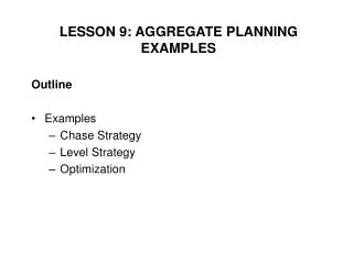
LESSON 8: AGGREGATE PLANNING. Outline Aggregate Planning Issues Costs Two Strategies Chase Strategy Level Strategy Optimization. Aggregate Production Planning.

E N D
LESSON 8: AGGREGATE PLANNING Outline • Aggregate Planning • Issues • Costs • Two Strategies • Chase Strategy • Level Strategy • Optimization
Aggregate Production Planning • Chapter 2 discusses forecasting. If the demand for a product changes over time, we need to plan the resource capacity the firm will need over time. • Aggregate production planning determines the resource capacity a firm may need to meet its demand. • Aggregate production planning is a short term decision making process. The planning horizon is typically 6 to 12 months. • Since the planning horizon is short, it is usually not feasible to build or shut down plants, purchase or sell equipment, etc.
Aggregate Production Planning • However, capacity may be adjusted in some other ways. It is usually possible to • hire or lay off workers • increase or decrease number of shifts • increase or decrease number of working days in a week • increase or decrease working hours (overtime or undertime) • subcontract work to other firms • build up or deplete inventory levels • Aggregate production planning meets the requirement of resource capacity using the above.
Aggregate Production Planning • The term aggregate refers to the fact that the plan is developed for a line of products, not just one individual product. For example, suppose that a firm produces three types of chairs: ladder-back chair, kitchen chair and desk chair. If an aggregate production plan is required for the chairs, the plan may consider an aggregate unit of chair. It will specify how many aggregate units of chair will be produced in various planning periods. • An aggregate unit is some kind of an “average” unit. Different products of the same product line may require different amount of worker/machine time, raw materials, etc. and their selling prices may also be different. It is not always very obvious what the aggregating scheme should be.
Aggregate Production Planning • An example of an aggregation scheme is given in Example 3.1, pp. 114-115 of the text. A firm produces 6 different models of washing machines Model Working Individual/Total Sales Number Hours Required Ratio A5532 4.2 0.32 K4242 4.9 0.21L9898 5.1 0.17 L3800 5.2 0.14 M2624 5.4 0.10 M3880 5.8 0.06
Aggregate Production Planning • The manager decides to define an aggregate unit of production as a fictitious machine requiring some weighted total working hours where the weights are taken from the individual/total sales ratio given in the previous slide. 0.32(4.2) + 0.21(4.9) + 0.17(5.1) + 0.14(5.2) + 0.10(5.4) + 0.06(5.8) = 4.856 hours
Hierarchy of Production Decisions • The next slide presents a schematic view of the aggregate production planning function and its place in the hierarchy of the production planning decisions. • Forecasting: First, a firm must forecast demand for aggregate sales over the planning horizon. • Aggregate planning: The forecasts provide inputs for determining aggregate production and workforce levels over the planning horizon. • Master production schedule (MPS): Recall, that the aggregate production plan does not consider any “real” product but a “fictitious” aggregate product. The MPS translates the aggregate plan output in terms of specific production goals by product and time period. For example,
Hierarchy of Production Decisions suppose that a firm produces three types of chairs: ladder-back chair, kitchen chair and desk chair. The aggregate production considers a fictitious aggregate unit of chair and find that the firm should produce 550 units of chairs in April. The MPS then translates this output in terms of three product types and four work-weeks in April. The MPS suggests that the firm produce 200 units of desk chairs in Week 1, 150 units of ladder-back chair in Week 2, and 200 units of kitchen chairs in Week 3. • Material Requirements Planning (MRP): A product is manufactured from some components or subassemblies. For example a chair may require two back legs, two front legs, 4 leg supports, etc. While forecasting, aggregate plan
Hierarchy of Production DecisionsMaster Production Schedule April May 1 2 3 4 5 6 7 8 Ladder-back chair 150 150 200 Kitchen chair 120 120 Desk chair 200 200 200 Aggregate production plan 790 550 for chair family
Hierarchy of Production Decisions and MPS consider the volume of finished products, MRP plans for the components, and subassemblies. A firm may obtain the components by in-house production or purchasing. MRP prepares a plan of in-house production or purchasing requirements of components and subassemblies. • Scheduling: Scheduling allocates resource over times in order to produce the products. The resources include workers, machines and tools. • Vehicle Routing: After the products are produced, the firm may deliver the products to some other manufacturers, or warehouses. The vehicle routing allocates vehicles and prepares a route for each vehicle.
Hierarchy of Production DecisionsMaterials Requirement Planning Back slats Seat cushion Leg supports Seat-frame boards Back legs Front legs
Issues in Aggregate Planning • Smoothing • Smoothing refers to costs that result from changing workforce level • Two of the key components of smoothing costs are costs associated with hiring and firing workers • Firing workers could have far-reaching consequences and the costs may be difficult to evaluate • Bottleneck problems • Bottleneck refers to the inability of the system to respond to sudden changes in demand • For example, a bottleneck may arise if the demand in one month is suddenly so high that the plant does not have sufficient capacity to meet the demand
Issues in Aggregate Planning • Planning horizon • Inaccurate forecasts are associated with too large planning horizon and planning may be ineffective with too small planning horizon • To minimize the inventory holding cost during the planning horizon, the aggregate plan may recommend zero inventory at the end of the planning horizon. This is known as the end-of-horizon effect. This may be a poor strategy, specially if demand increases at that time. • Often, rolling schedules are used. In a rolling schedule, a plan is prepared for several periods more than the planning horizon over which the plan will be
Issues in Aggregate Planning implemented. At the time of the next decision, a new forecast is appended and old forecasts may be revised. The new plan may recommend different production and workforce levels than were recommended earlier. • Often, it desired that because of production lead times that the schedule be frozen for a certain number of planning periods. Then, production and workforce levels over the frozen horizons cannot be changed. • Nature of Demand • Aggregate planning ignores the possibility of forecast errors. Assuming deterministic demand, aggregate planning can incorporate seasonal fluctuations and business cycles into the planning function.
Aggregate Production Planning • Input • Demand forecast • Level of resources available • Relevant cost information • Output • Aggregate production quantities • production, inventory, backorder • Level of resources needed • Workforce, overtime, machine capacity level, subcontracting
Costs in Aggregate Planning • Smoothing costs • Hiring costs • Time and cost to advertise positions • Interview candidates • Train new recruits • Firing costs • Severance pay • The costs of a decline in worker morale • The potential for decreasing the size of the labor pool in the future
Costs in Aggregate Planning • Inventory holding costs • Opportunity cost of capital • Cost of storage space • Taxes and insurance against fire, theft, and other losses • Breakage, spoilage, deterioration and obsolescence • Example of calculation of inventory holding costs Cost of capital - 15% Taxes and insurance - 2% Storage - 5% Breakage/spoilage - 3% Total - 25%
Costs in Aggregate Planning • Shortage costs • Shortages occur when the demand exceeds the production capacity. One of two types of costs is charged depending on whether a shortage results in loss of sales or not: • Backorder - if the excess demand is backlogged and fulfilled in a future period, backorder cost is charged (bookkeeping and/or delay costs). • Lost sales - if the excess demand is lost because the customer goes elsewhere, the lost sales is charged. The lost sales include goodwill and loss profit margin (=selling price - unit variable cost)
Costs in Aggregate Planning Inventory Holding and Shortage Costs
Costs in Aggregate Planning • Production costs • Straight time costs • Labor costs, regular time ($/hour) • Overtime and subcontracting costs • Labor costs, overtime costs ($/hour) • Cost of subcontracting ($/unit or $/hour) • Idle time costs • In most contexts, the idle time cost is zero. • However, a non-zero cost is appropriate if idle time has some consequences. For example, when aggregate units are inputs to another process, idle times may delay the process.
A Feasible Aggregate Plan • The next slide shows a chart in which cumulative number of units are plotted over a planning horizon. • There are two lines: • Production line: this line corresponds to the production schedule and shows the cumulative number of units produced • Demand line: this line corresponds to the demand and shows the cumulative net demand • The production line is straight and its slope does not change. This means that a constant number of units is produced in every period.
A Feasible Aggregate Plan • The production planning strategy in which a constant number of units is produced in each period is called the level strategy. Hence, the chart shows a level strategy. • The demand line is not straight. This means that the demand is different in different period. • At any point of time, the difference between cumulative production and cumulative net demand is the inventory. Hence, the vertical difference shows the inventory. • If shortages are not allowed, a production schedule is feasible if the production line is always above the demand line. Hence, the chart shows a feasible production schedule.
A Feasible Aggregate Plan • If the production line lies below the demand line, the inventory is negative and shortages take place. Such a production schedule can also be feasible if shortages are allowed. • Both the lines meet in the end of the planning horizon. That means that the inventory is zero at the end of the planning horizon. This is the end-of -horizon effect discussed before. It is is not necessary to have a zero inventory at the end of the planning horizon and sometimes it is undesirable. If there is a positive inventory at the end of the planning horizon, there will be a gap between the production and demand lines at the end of the planning horizon.
A Feasible Aggregate Plan • If shortages are allowed, the production line may lie above or below the demand line. When the production line is above the demand line, inventory is positive and when the production line is below the demand line, inventory is negative. • The opposite of the level strategy is the chase strategy. In a chase strategy the production volume is the same as the demand. So, the inventory is always zero. In such a case, there is no gap between the production line and the demand line.
Constraints • Sometimes decision making can be constrained by • limits on overtime • limits on layoffs • limits on capital available • limits on stockouts and backorders
READING AND EXERCISES Lesson 8 Reading: Section 3.1 - 3.3 , pp. 113-120 (4th Ed.), pp. 108-117 (5th Ed.) Exercise: 8, p. 121 (4th Ed.), p. 117 (5th Ed.)