Quantitative Variables

1. Quantitative Variables • Recall that quantitative variables have units, and are measured on a continuous scale… • Examples: income (in $), height (in inches), website popularity (by number if hits)

2. Quantitative Variables • Mathematical operations on quantitative variables makes sense … • Adding, subtracting, taking the arithmetic average etc…

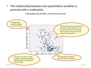
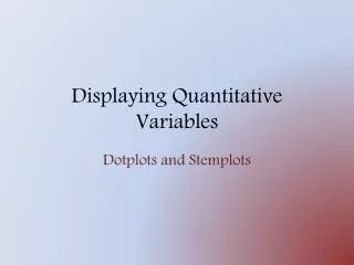
3. Visualizing quantitative variables • Histogram – note that the bars touch each other – the values at the bottom are continuous!

4. Visualizing quantitative variables • Dot plot

5. So why visualize? • To see the features of the data • Shape • Center • Spread

6. Constructing a Histogram

7. Step 1 – Choose the Classes

8. Step 2 – Count

9. Step 3 – Draw the Histogram

10. Identifying Identifiers • Identifier variables are categorical variables with exactly one individual in each category. • Examples: Social Security Number, ISBN, FedEx Tracking Number • Don’t be tempted to analyze identifier variables. • Be careful not to consider all variables with one case per category, like year, as identifier variables. • The Why will help you decide how to treat identifier variables.

11. Shape - Modality and Symmetry

12. Humps and Bumps • Does the histogram have a single, central hump or several separated bumps? • Humps in a histogram are called modes. • A histogram with one main peak is dubbed unimodal; histograms with two peaks are bimodal; histograms with three or more peaks are called multimodal.

13. A bimodal histogram has two apparent peaks: Humps and Bumps (cont.)

14. A histogram that doesn’t appear to have any mode and in which all the bars are approximately the same height is called uniform: Humps and Bumps (cont.)

15. Symmetry • Is the histogram symmetric? • If you can fold the histogram along a vertical line through the middle and have the edges match pretty closely, the histogram is symmetric.

16. Symmetry (cont.) • The (usually) thinner ends of a distribution are called the tails. If one tail stretches out farther than the other, the histogram is said to be skewed to the side of the longer tail. • In the figure below, the histogram on the left is said to be skewed left, while the histogram on the right is said to be skewed right.

17. Anything Unusual? • Do any unusual features stick out? • Sometimes it’s the unusual features that tell us something interesting or exciting about the data. • You should always mention any stragglers, or outliers, that stand off away from the body of the distribution. • Are there any gaps in the distribution? If so, we might have data from more than one group.

18. Anything Unusual? (cont.) • The following histogram has outliers—there are three cities in the leftmost bar:

19. Shape - Outliers Do any unusual features stick out? We will discuss these in more detail when we introduce box plots.

20. Why do we care about shape? • When quantitative variables are skewed, we describe the center and spread using different measures than if the variable is symmetric.

21. The center of the distribution - median • The “most typical value” in the data usually refers to some measure of the “center” of the distribution • The median is the point that divides the histogram into two equal pieces

22. Calculating the median • First, order all values from smallest to largest • Let n = sample size • If n is odd, the median is located at the (n+1)/2 position • If n is even, the median is the average of the two middle points

23. Calculating the median • Example 1 : Earthquakes in N.Z. • 2010 EQ magnitudes in N.Z.: 3.2,3.2,3.3,3.4,3.5,3.5,3.6,3.6, 3.7, 3.8,3.9,3.9,6.4 • Since n is odd: • Median is located at the (n+1)/2 = (13+1)/2 = 7th position • Median is 3.6

24. Calculating the median • Example 2 : Earthquakes in Samoa • 2010 Earthquake magnitudes in Samoa: 1.1,3.5,4.4,4.6,5.1,6.0 • Since n is even: • Median is the average of • (n/2) = (6/2) = 3rd value (4.4) • (n/2)+1 = (6/2)+1 = 4th value (4.6) • Median is (4.4+4.6)/2 = 4.5

25. Median - Interpretation • Example 1: The typical earthquake size in Fiji in 2010 was 3.6 on the Richter scale • How useful is this?

26. Spread • If all earthquakes in Fiji were 3.6, then the Median would be sufficient information • But they are not, so we need to see how spread out are the earthquakes around 3.6

27. Spread - Range • Range = max value - min value • For the Fiji example: • Range = 6.4-3.2 = 3.2 • This is not useful…why?

28. Spread-IQR • Inter-quartile range • IQR = Q3 - Q1 • Q1 = Median of 1st half • Q3 = Median of 2nd half • One single number that captures “how spread out the data is”

29. Spread-IQR • NZ Earthquake example cont: • 2010 EQ magnitudes in N.Z. (divided): 1st half: 3.2,3.2,3.3,3.4,3.5,3.5,3.6, 2nd half: 3.6, 3.6, 3.7,3.8,3.9,3.9,6.4 • Q1 = (n+1)/2 = (7+1)/2 = 4 -> 3.4 • Q3 = (n+1)/2 = (7+1)/2 = 4 -> 3.8 • IQR = 3.8-3.4 = 0.4 • When n is odd, include median in both lists…don’t when n is even

30. IQR • Almost always a reasonable summary of the spread of a distribution • Shows how spread out the middle 50% of the data is • One problem is that it ignores a lot of individual variation

31. 5-Number Summary • Minimum • Q1 • Median • Q3 • Maximum

32. The five-number summary of a distribution reports its median, quartiles, and extremes (maximum and minimum). Example: The five-number summary for the ages at death for rock concert goers who died from being crushed is The Five-Number Summary

33. Categorical or Quantitative?