Download
1 / 50
530 likes | 688 Vues
“Theory of Storage and Option Pricing: Determinants of Implied Skewness and Kurtosis. Marin Bozic and T. Randall Fortenbery University of Wisconsin-Madison Znanstveni utorak , Ekonomski Institut Zagreb 15 lipanj , 2010. Types of uncertainty: production risk

E N D
“Theory of Storage and Option Pricing: Determinants of Implied Skewness and Kurtosis Marin Bozic and T. Randall Fortenbery University of Wisconsin-Madison Znanstveniutorak, EkonomskiInstitut Zagreb 15 lipanj, 2010
Types of uncertainty: • production risk • price risk (input and output) • counterparty risk • cash flow risk • What can be done about it: • “Take it easy approach” a.k.a. Do Nothing, sell for cash • Removing price risk but forfeiting opportunity as well: Hedging with futures • Removing downside risk, but preserving opportunity of favorable price change: Options!
Futures contract: A promise to sell (or buy) at a pre-specified quantity, price, location, and time in the future (“delivery month”) • removes (almost all) price risk • removes counterparty risk • removes the opportunity to make some extra profit if prices increase a lot • Options contract: Gives holder a right, but not the obligation to sell (or buy) a futures contract with pre-specified quantity, at a pre-specified price (strike price), at any point before the delivery month. • unlike futures, does not remove the profit opportunity from favorable cash prices • unlike futures, it’s not “free”, you have to pay for the right upfront
We entered a Dec’ 10 futures contract Promising to sell at a price of $3.70. Price is locked, no matter what.
On 2/1/2010 we bought an option To sell at the price of $3.70. If futures price in June is better than that, we forfeit the option. If not, we exercise it.
Option is never the best choice (ex post) But it’s rarely the worst.
Options are a sort of insurance. In good times you don’t exercise it, in bad times it may save your business. • If farmers are risk-averse, they will likely hedge to reduce the uncertainty. • Does that mean that price of options depend on risk-preferences of farmers? Not necessarily. In fact, some folks got the Nobel price for showing how price of options are arrived at, solely by arbitraging away riskless profits.
Merton (1973), Black & Scholes (1973), Black (1976) • Arbitrage Pricing Theory: • Start from reasonable if simplifying assumptions: • Prices can never be negative • Changes in prices are proportional to time passed • It is known how small change in price will affect the price of option • key assumptions: normality, volatility assumed constant and independent of price level (1)
Black & Scholes do a nice trick to show that if an arbitrageur holds cleverly chosen proportions of options and underlying futures, then in the simple world described by Eq. (1) such portfolio may be made riskless. • Returns on riskless portfolio must match riskless rate of interest (holding treasury bills) and hence risk preferences are purged from the function determining price. (2)
In reality, we do not observe volatility parameter directly. • However, we can invert the function by asking: which would produce the option prices we do observe, if Black’s model assumptions hold • Calculated option prices via Black-Scholes formula • T-t = 90/365 r = 5.32% • σ = 36.1% Ft = $3.64 • Pretended we don’t know σ and estimated it via Newton-Raphson algorithm, for each strike price separately • Key consequence of the theory: IV curve should be flat!
USDA Crop reports “XXX”, published 15th of March, June, Sep, Dec • Intention to plant reports • Planted reports • harvest reports
Implied Volatility curve can also be convex and symmetric. • That’s why we usually call IV curves “Volatility smiles” Source: Hull, J.C. (2006) – Options, Futures, and Other Derivatives, pg. 377
vs. • How can we replicate the results? • Can we explain the anomalies? • Two basic approaches • Work from the beginning: Enrich the stochastic process • for underlying asset: • make σ dependent on F, or even stochastic itself; introduce “jumps” • 2. Work from the end: Treat option as “risk-neutral expectation of terminal payoff” • enrich the terminal distribution of the futures price directly
Theory implies terminal distribution of futures price is log-normal • (Log-normal = log of terminal price is normally distributed) • If the traders expect terminal distribution to be non-normal, option prices will reflect that. Implied volatility curve will not be flat.
For a standardized density: location spread asymmetry tail behavior
Kurtosis Skewness Source: Rubinstein, M. (1998) Edgeworth Binomial Trees
Calculated option prices via Edgeworth binomial tree • T-t = 90/365 r = 5.32% • σ = 36.1% Ft = $3.64 • Pretended we don’t know σ and estimated it via Newton-Raphson algorithm for each strike price separately, assuming Black’s model holds (S=0, K=3). • Key consequences of non-normal kurtosis: • Volatility Smiles! • Higher kurtosis • Deeper smile
Calculated option prices via Edgeworth binomial tree • T-t = 90/365 r = 5.32% • σ = 36.1% Ft = $3.64 • Pretended we don’t know σ and estimated it via Newton-Raphson algorithm for each strike price separately, assuming Black’s model holds (S=0, K=3). • Key consequences of negative skewness: • Downward sloping curve! • Stronger skewness • Deeper slope
Date: Jun 26, 2006 Contract: Corn, Dec ’06 Futures Price: $2.49 Commodities tend to have positively sloped implied volatility curve. Our research will explain why.
Calculated option prices via Edgeworth binomial tree • T-t = 90/365 r = 5.32% • σ = 36.1% Ft = $3.64 • Pretended we don’t know σ and estimated it via Newton-Raphson algorithm for each strike price separately, assuming Black’s model holds (S=0, K=3). • Key consequences of positive skewness: • Upward sloping curve! • Stronger skewness • Deeper slope
The higher the skewness of the terminal distribution is, the higher will be the difference between implied volatility for options low and high strikes. • But Edgeworth can only create up to 8-9 percentage point difference, while we observe 15% difference in IV, or even more. • If we try to push Edgeworth harder, approximation will fail, density may turn negative in tails • We needed a different method to approach non-normality of terminal log-prices…
We needed a distribution that would… • allow for high flexibility in first four moments four-parameter family • Would be easy to simulate closed form percentile function (inverse CDF) • would produce close-form solution to option pricing
1. Flexibility: by tweaking parameters of the distribution, we can accommodate almost any desired shape. Alternatively, we can think of this as being able to approximate any other distribution up to first four moments
2. Easy to simulate: closed form inverse CDF allows easy drawing from GLD with arbitrary shape. • Problem: parameters correspond to moments in highly complicated way
2. Easy to simulate: closed form inverse CDF allows easy drawing from GLD with arbitrary shape. • Problem: parameters correspond to moments in highly complicated way
2. Easy to simulate: closed form inverse CDF allows easy drawing from GLD with arbitrary shape. • Problem: parameters correspond to moments in highly complicated way
2. Easy to simulate: closed form inverse CDF allows easy drawing from GLD with arbitrary shape. • Problem: parameters correspond to moments in highly complicated way
2. Easy to simulate: closed form inverse CDF allows easy drawing from GLD with arbitrary shape. • Problem: parameters correspond to moments in highly complicated way
Black-Scholes formula for European call on non-dividend paying stock: GLD formula for European call on futures contract
Date: Jun 26, 2006 Contract: Corn, Dec ’06 Futures Price: $2.49 Commodities tend to have positively sloped implied volatility curve. Our research will explain why.
Essential role of storage • Imagine that a corn yield is normally distributed. I.e. it’s equally likely that harvest will be better than usual and that it will be worse than usual. • If harvest is very good, we don’t have to eat it all right away, we can store it • If harvest is bad, we have only so much of last crop’s stocks we can use in addition to new crop. • Normal shocks to yield will lead to skewed shocks to price!
Tighter market • Higher expected price • Larger variance • Higher (more positive) skewness Source: Williams & Wright (1991) Storage and Commodity Markets
Literature has worked out that rational expectations competitive model is able to replicate time-series properties of spot commodity price: mean-reversion, sudden peaks with gradual decline, skewness • We were not able to test so far if market expectations were in alignment with that model • We propose here a way to test exactly this: • if model works, then in periods where inventories are low, and buffers to bad harvest are less effective, market should expect higher skewness in terminal price distribution.
Tick data for futures and options for corn, wheat and soybeans for 1995-2009, donated by Chicago Mercantile Exchange: 90+ million data points • Options matched with last observed futures trade • Frequency reduced to 15 minutes interval • 11,139 files. • For each option, implied volatility calculated using Black’s model modified to account for early exercise (Cox Ross Rubinstein binomial trees, 500 steps) • Price of equivalent European option calculated
Major role USDA reports play: • Quarterly stock reports • “Grain Stocks”, Jan 11, Mar 31, Jun 30, Sep 30 • USDA surveys on intended acres planted • “Prospective plantings”, March 31 • Report on actual acres planted • “Acreage”, June 30 • Report on how crops are progressing • “Crop progress”, weekly (Monday, 4pm), Apr-Dec
Months traded: March, May, July, September, December • Contract size: 5000 bushels • Options expire: The last Friday preceding the first day of the delivery month by at least two business days. • June, 14 2010, closing prices: • December 2010 Futures: 3.72 $/bu • Options: • $3.60 Call: $0.355 ($1,775 per contract) • $3.90 Put: $0.397 ($1,985 per contract)
Lower ending stocks relative to demand are associated with higher difference in implied volatility between high and low strike prices
Corn • Dec ’09
Used least squares to estimate lambda parameters that best match • Observed option prices for a certain contract on a given day • * Software used: excel solver, Fortran .dll libraries for • computationally intensive elements • * Results may be sensitive to starting values • * calculated implied skewness and kurtosis for Corn • December contracts, as priced from June, 10 to June, 20 of • each year (i.e. before Acreage report) • * averaged implied moments over that 9 trading days
Implied skewness regressed on intended increase in planted acreage and ending stocks-to-use • if hypothesis has any merit, we should see statistically significant, negative parameters for both explanatory variables.
Deviations from classical Black’s model can be explained by theory of storage – asymmetric response of price to symmetric shocks to crop yield under rational expectations induces expected terminal distribution to be positively skewed and leptokurtic to the extent that exceeds skewness and kurtosis of lognormal distribution • We find the way to extend the test of rational expectations competitive model from time-series properties of spot price to market expectations of future spot price • Next challenge: try to separate option premium due to market expectations from “liquidity premium” priced in options that are very much out-of-money, and are thinly traded.
Thank You! ______________________________________________________________ Theory of Storage and Option Pricing: Determinants of Implied Skewness and Kurtosis Marin Bozic and T. Randall Fortenbery University of Wisconsin-Madison Contact Info: Marin Bozic Research Assistant Department of Agricultural and Applied Economics University of Wisconsin-Madison Email: bozic@wisc.edu