Download
1 / 11
110 likes | 244 Vues
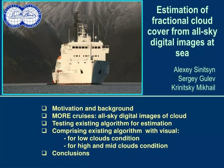
Estimation of fractional cloud cover from all-sky digital images at sea. Alexey Sinitsyn Sergey Gulev Krinitsky Mikhail. Motivation and background MORE cruises: all-sky digital images of cloud Testing existing algorithm for estimation Comprising existing algorithm with visual:

E N D
Estimation of fractional cloud cover from all-sky digital images at sea Alexey Sinitsyn Sergey Gulev Krinitsky Mikhail • Motivation and background • MORE cruises: all-sky digital images of cloud • Testing existing algorithm for estimation • Comprising existing algorithm with visual: - for low clouds condition - for high and mid clouds condition • Conclusions
Motivation: • Accurate estimation of cloud fraction is critical for the quantitative computation of surface short wave and long • wave solar radiation at sea. • Today science advanced to a point when we can engage information about cloud types in the analysis of solar radiation considerably extending the abilities of routine observations of cloud fraction taken visually. • This is particularly important under overcast conditions frequently associated with the mixed cloud types and, therefore, optical thickness of the cloudy atmosphere
MORE cruises: 2007-2010 (for all-sky image) Days • October 2007 R/V “Academician Ioffe”Santa Cruz (Spain) –Montevideo (Uruguay) • October – November 2009 R/V “Academician Ioffe” Kaliningrad (Russia) – CapeTown (RSA) • September 2010 R/V “Academician Ioffe” cape Farewell (Greenland) – Szczecin (Poland) • 18 • 31 • 15
Sigma 8mm F3,5 EX DG Circular-Fisheye All-sky image package • Nikon D80 with 10,2 effective pixels • Sigma 8mm F3,5 Circular-Fisheye • Angle of view for APS-C sensor 180 ° х 120 ° • Projection of fisheye lens is equidistant projection • All shoots were taken with hands Example of all-sky digital image • Data collected: 2007-2010: • 62 days of all-sky digital images with 1-hour resolution • Simulteneous hourly observations of standard meteorological variables (clouds, air temperature, humidity, SST)
Existing algorithm for cloud recognizing (i) Sky Index for Yamashita M.and etc, 2004: Sky Index (SI) = (DNBlue – DNRed) / (DNBlue + DNRed), DNBlue = digital number of blue channel DNRed = digital number of red channel Empirical threshold 0,1. If SI <= 0,1 then consider pixel as cloudy (ii) Sky Index forKalisch J., Macke A. (IFM-GEOMAR), 2008: Sky Index (IFM SI) = (DNRed) / (DNBlue ), DNBlue = digital number of blue channel DNRed = digital number of red channel Empirical threshold 0,8. If SI > 0,8 then consider pixel as cloudy
Comparisons of the algorithm cloud cover estimation for batch processing Applied to batch processing both algorithm for cloud estimation shown same result. Corr = 0.99 Stddev = 0.19
Comparisons of the SI algorithm cloud cover estimation with visual data 2009 Corr = 0.84 Stddev = 1.89 2007 Corr = 0.79 Stddev = 2.11 2010 Corr = 0.78 Stddev = 1.80
Comparison of calculations with observations in the case of low clouds 2009 Corr = 0.92 Stddev = 1.97 2007 Corr = 0.92 Stddev = 1.97 2010 Corr = 0.77 Stddev = 1.87
Comparison of calculations with observations in the case of high and mid clouds 2007 Corr = 0.69 Stddev = 2.81 2007 Corr = 0.84 Stddev = 2.10
Potential causes of errors 20% of FOV = 2 cloud amount Rigid threshold
Conclusions: • Using these parameters retrieved from the sky images we improve the accuracy of computation of cloud dependent radiative fluxes at sea surface. • Use only one threshold value - incorrectly. Within each series of photos needed correction threshold. • For further work with the cloud amount and the type of cloud we need to use Circular-Fisheye for crop matrix.