Download
1 / 32
330 likes | 851 Vues
Optical Flow. Donald Tanguay June 12, 2002. Outline. Description of optical flow General techniques Specific methods Horn and Schunck (regularization) Lucas and Kanade (least squares) Anandan (correlation) Fleet and Jepson (phase) Performance results. Optical Flow.

E N D
Optical Flow Donald TanguayJune 12, 2002
Outline • Description of optical flow • General techniques • Specific methods • Horn and Schunck (regularization) • Lucas and Kanade (least squares) • Anandan (correlation) • Fleet and Jepson (phase) • Performance results
Optical Flow • Motion field – projection of 3-D velocity field onto image plane • Optical flow – estimation of motion field • Causes for discrepancy: • aperture problem: locally degenerate texture • single motion assumption • temporal aliasing: low frame rate, large motion • spatial aliasing: camera sensor • image noise
Brightness Constancy Image intensity is roughly constant over short intervals: Taylor series expansion: Optical flow constraint equation: (a.k.a. BCCE: brightness constancy constraint equation) (a.k.a. image brightness constancy equation)(a.k.a. intensity flow equation)
Aperture Problem One equation in two unknowns => a line of solutions
Aperture Problem In degenerate local regions, only the normal velocity is measurable.
General Techniques • Multiconstraint • Hierarchical • Multiple motions • Temporal refinement • Confidence measures
General Techniques • Multiconstraint • over-constrained system of linear equations for the velocity at a single image point • least squares, total least squares solutions • Hierarchical • coarse to fine • help deal with large motions, sampling problems • image warping helps registration at diff. scales
Multiple Motions • Typically caused by occlusion • Motion discontinuity violates smoothness, differentiability assumptions • Approaches • line processes to model motion discontinuities • “oriented smoothness” constraint • mixed velocity distributions
Temporal Refinement • Benefits: • accuracy improved by temporal integration • efficient incremental update methods • ability to adapt to discontinuous optical flow • Approaches: • temporal continuity to predict velocities • Kalman filter to reduce uncertainty of estimates • low-pass recursive filters
Confidence Measures • Determine unreliable velocity estimates • Yield sparser velocity field • Examples: • condition number • Gaussian curvature (determinant of Hessian) • magnitude of local image gradient
Specific Methods • Intensity-based differential • Horn and Schunck • Lucas and Kanade • Region-based matching (stereo-like) • Anandan • Frequency-based • Fleet and Jepson
Horn and Schunck Minimize the error functional over domain D: smoothnessterm BCCE smoothnessinfluenceparameter Solve for velocity by iterating over Gauss-Seidel equations:
Horn and Schunck • Assumptions • brightness constancy • neighboring velocities are nearly identical • Properties + incorporates global information + image first derivatives only • iterative • smoothes across motion boundaries
Lucas and Kanade Minimize error via weighted least squares: which has a solution of the form:
Lucas and Kanade • Assumptions • locally constant velocity • Properties + closed form solution - estimation across motion boundaries
Anandan • Laplacian pyramid – allows large displacements, enhances edges • Coarse-to-fine SSD matching strategy
Anandan • Assumptions • displacements are integer values • Properties + hierarchical + no need to calculate derivatives • gross errors arise from aliasing - inability to handle subpixel motion
Fleet and Jepson A phase-based differential technique. Complex-valued band-pass filters: Velocity normal to level phase contours: Phase derivatives:
Fleet and Jepson • Properties: + single scale gives good results - instabilities at phase singularities must be detected
Image Data Sets • SRI sequence: Camera translates to the right; large amount of occlusion; image velocities as large as 2 pixels/frame. • NASA sequence: Camera moves towards Coke can; image velocities are typically less than one pixel/frame. • Rotating Rubik cube: Cube rotates counter-clockwise on turntable; velocities from 0.2 to 2.0 pixels/frame. • Hamburg taxi: Four moving objects – taxi, car, van, and pedestrian at 1.0, 3.0, 3.0, 0.3 pixels/frame
References Anandan, “A computational framework and an algorithm for the measurement of visual motion,” IJCV vol. 2, pp. 283-310, 1989. Barron, Fleet, and Beauchemin, “Performance of Optical Flow Techniques,” IJCV 12:1, pp. 43-77, 1994. Beauchemin and Barron, “The Computation of Optical Flow,” ACM Computing Surveys, 27:3, pp. 433-467, 1995. Fleet and Jepson, “Computation of component image velocity from local phase information,” IJCV, vol. 5, pp. 77-104, 1990.
References Heeger, “Optical flow using spatiotemporal filters,” IJCV, vol. 1, pp. 279-302, 1988. Horn and Schunck, “Determining Optical Flow,” Artificial Intelligence, vol. 17, pp. 185-204, 1981. Lucas and Kanade, “An iterative image registration technique with an application to stereo vision,” Proc. DARPA Image Understanding Workshop, pp. 121-130, 1981. Singh, “An estimation-theoretic framework for image-flow computation,” Proc. IEEE ICCV, pp. 168-177, 1990.