Download
1 / 33
520 likes | 1.16k Vues
Introduction to Optimization. CSC105 PowerPoint Presentation by Peggy Batchelor, Furman University. Learning Objectives. Recognize decision-making situations which that may benefit from an optimization modeling approach. Formulate algebraic models for linear programming problems.

E N D
Introduction to Optimization CSC105 PowerPoint Presentation by Peggy Batchelor, Furman University
Learning Objectives • Recognize decision-making situations which that may benefit from an optimization modeling approach. • Formulate algebraic models for linear programming problems. • Develop spreadsheet models for linear programming problems. • Use Excel’s Solver Add-In to solve linear programming problems. • Interpret the results of models and perform basic sensitivity analysis.
Optimization: Basic Ideas • Major field within the discipline of Data Analytics, Operations Research and Management Science • Optimization Problem Components • Decision Variables • Objective Function (to maximize or minimize) • Constraints (requirements or limitations) • Basic Idea • Find the values of the decision variables that maximize (minimize) the objective function value, while staying within the constraints.
Linear Programming (LP) • If the objective function and all constraints are linear functions of the decision variables (e.g., no squared terms, trigonometric functions, ratios of variables), then the problem is called a Linear Programming (LP) problem. LPs are much easier to solve by computer than problems involving nonlinear functions. • Real-world LPs are solved which contain hundreds of thousands to millions of variables (with specialized software!). Our problems are obviously much smaller, but the basic concepts are much the same.
Real-World Examples • Dynamic and Customized Pricing • Product Mix • Scheduling/Allocation • Routing/Logistics • Supply Chain Optimization • Facility Location • Financial Planning/Asset Management • Etc.
Solving Optimization Problems • Understand the problem; draw a diagram • Write a problem formulation in words • Write the algebraic formulation of the problem • Define the decision variables • Write the objective function in terms of the decision variables • Write the constraints in terms of the decision variables
Solving Optimization Problems (continued) • Develop Spreadsheet Model • Set up the Solver settings and solve the problem • Examine results, make corrections to model and/or Solver settings • Interpret the results and draw insights
Solver • We will use Solver, an Excel add-in, to solve Linear Programming problems. • Add-In: An additional piece of software that Excel loads into memory when needed. • In Excel, go to FileOptions Add-ins, click Go at bottom of dialog box • After choosing Solver in the Add-Ins list, go to Data tabSolver to access Solver.
Example: Product Mix Decision • DJJ Enterprises makes automotive parts, Camshafts & Gears • Unit Profit: Camshafts $25/unit, Gears $18/unit • Resources needed: Steel, Labor, Machine Time. In total, 5000 lbs steel available, 1500 hours labor, and 1000 hours machine time. • Camshafts need 5 lbs steel, 1 hour labor, 3 hours machine time. • Gears need 8 lbs steel, 4 hours labor, 2 hours machine time. • How many camshafts & gears to make in order to maximize profit?
Understanding the Problem • Text-Based Formulation • Decision Variables: Number of camshafts to make, number of gears to make • Objective Function: Maximize profit • Constraints: Don’t exceed amounts available of steel, labor, and machine time.
Algebraic Formulation • Decision Variables • C = number of camshafts to make • G = number of gears to make • Objective Function • Maximize 25C + 18G (profit in $) • Constraints • 5C + 8G <= 5000 (steel in lbs) • 1C + 4G <= 1500 (labor in hours) • 3C + 2G <= 1000 (machine time in hours) • C >= 0, G >= 0 (non-negativity)
Important Concepts • Linear Program: The objective function and constraint are linear functions of the decision variables. Therefore, this is a Linear Program. • Feasibility • Feasible Solution. A solution is feasible for an LP if all constraints are satisfied. • Infeasible Solution. A solution is infeasible if one or more constraints is violated. • Check the solutions C=75, G=200; and C=300, G=200 for feasibility. • Optimal Solution. The optimal solution is the feasible solution with the largest (for a max problem) objective value (smallest for a min problem).
Solving Linear Programming Problems • Trial and error: possible for very small problems; virtually impossible for large problems. • Graphical approach: It is possible to solve a 2-variable problem graphically to find the optimal solution (not shown). • Simplex Method. This is a mathematical approach developed by George Dantzig. Can solve small problems by hand. • Computer Software. Most optimization software actually uses the Simplex Method to solve the problems. Excel’s Solver Add-In is an example of such software. • Solver can solve LPs of up to 200 variables. Enhanced versions of Solver are available from Frontline Systems (http://www.solver.com).
Spreadsheet Model Development • Develop correct, flexible, documented model. • Sections for decision variables, objective function, and constraints. • Use algebraic formulation and natural structure of the problem to guide structure of the spreadsheet. • Use one cell for each decision variable • Store objective function coefficients in separate cells, and use another cell to compute the objective function value. • Store constraint coefficients in cells, compute the LHS value of each constraint, for comparison to the RHS value.
Spreadsheet Model • C=75, G=200 (cells B5:C5) entered as trial values. This is a feasible, but not the optimal, solution. • Note close relationship to algebraic formulation. • Note that only one distinct formula needed to be entered; once entered in Cell D8, it was copied to Cells D11:D13. • This is possible because the coefficients were stored separately in a specific structure.
Solver Basics • Don’t even think about using Solver until you have a working, flexible spreadsheet model that you can use as a “what if” tool! • Solver Settings • Specify Objective Cell (objective function) • Specify Changing Cells (decision variables) • Specify Constraints • Specify Solver Settings • Solve Problem to find Optimal Solution
Solver Settings: Target Cell and Changing Cells • Specify Target Cell: D8 • Equal to: Max • Changing Cells (decision variables) • B5:C5
Solver Settings: Constraints • Click “Add” to add constraints • Select LHS Cell (D11), relationship (<=), and RHS Cell (F11). • LHS Cell should contain a formula which computes the LHS Value of the constraint. • Typically, RHS Cell should contain a fixed value, but this is not absolutely required. • Repeat for the other two constraints (for labor and machine time). • OR use the range for the LHS and the RHS (see next slide)
Solver Options • Select Simples LP” • Tells Solver to use the Simplex Method, which is faster and is Solver’s default optimization method. • Check “Make unconstrained Variables Non-negative” • Tells Solver that the decision variables (B5:C5, representing the number of Camshafts and Gears) must be 0 in any feasible solution. • Leave other settings at their defaults.
Completed Solver Box • Click “Solve” to tell Solver to find the Optimal Solution.
Solver Results Box • Be sure to read message of box. The one shown indicates the optimal solution has been found. There are others that indicate other possible ending points (covered later). • Click on Reports desired before clicking OK. Reports covered later.
Solved Spreadsheet (Optimal Solution) • Optimal Solution: Make 100 camshafts, 350 gears. • Optimal Objective Value: $8800 profit. • Both pieces of information are important. Knowing the optimal objective value is useless without knowing how that value can be attained.
Interpreting the Solution • Which constraints are actively holding us back from making even more profit? • Binding Constraints: Constraints at the optimal solution with the LHS equal to the RHS; equivalently for a resource, a binding constraint is one in which all the resource is used up. • Labor (all 1500 hours used), Machine Time (all 1000 hours used). • Non-Binding Constraints • Steel: Have 5000 lbs available, but only need 3300 lbs for this solution. • What-If Analysis. Once the Spreadsheet and Solver model is set up, it is easy to change one or more input values and re-solve the problem. • This interactive use can be a very powerful way to use optimization.
Solution Reports • Solver can generate three solution reports • Answer Report • Sensitivity Report • Limits Report: Not covered here • The Answer Report presents in a standard format the Solver Settings and the optimal solution. • The Sensitivity Report shows what will happen if certain problem parameters are changed from their current values.
Answer Report Tightening a binding constraint can only worsen the objective function value, and loosening a binding constraint can only improve the objective function value. As such, once an optimal solution is found, managers can seek to improve that solution by finding ways to relax binding constraints. • Three sections: Objective Cell, Changing Cells, Constraints • “Final Value” indicates optimal solution • For each constraint, binding/non-binding status and “slack” (difference between LHS and RHS)…slack is zero for binding constraints. • Also note that the Solver Settings for Objective Cell, Changing Cells, and Constraints are reported here. This can be a useful debugging tool.
Sensitivity Report • Note two sections: Variable Cells and Constraints
Sensitivity Report (continued) • Constraint Section • Shadow Price: This is the amount the optimal objective value will change by if the RHS of the constraint is increased by one unit. • Units of shadow price: (objective function units/constraint units). Example: for the steel constraint, the units are $/lb; for the labor constraint, the units are $/hour. • Allowable Increase/Decrease: Provides the increase/decrease of the RHS of the constraint for which the shadow price stays the same; that is, the effect on the objective value stays the same in this range. • Example • Shadow Price of Machine Time is $8.20/hour, valid for an increase of 1416 hours or a decrease of 250 hours. • If we make 200 additional machine time hours available, profit can be increased by (200 hours)($8.20/hour) = $1640. • What is the shadow price of a non-binding constraint? Why? Will this always be the case?
Sensitivity Report (continued) • Variable Cells Section • Allowable Increase/Decrease: This is the amount the objective coefficient for a decision variable can be increased/decreased without changing the optimal solution. • Example • Gears currently have a profit of $18/unit (objective coefficient). • Allowable Increase/Decrease is $82 and $1.33, respectively. • Interpretation: As long as the unit profit for gears is between $16.67 and $100, the optimal solution (production plan) will be to make 100 camshafts and 350 gears. • Note: The optimal solution (production plan) stays the same within this range, but the optimal objective value (profit) changes since the unit profit is changing. So, if the profit on gears goes up to $20/unit, profit will increase by ($20-$18)(350) = $700.
Sensitivity Report: Caveat! • Effects identified in the Sensitivity Report need to be carefully interpreted. • Specifically, the effect of the change of one parameter (e.g., a RHS value or an objective coefficient) assume that all other parameters of the model stay at their base case values. • For example, the Sensitivity Report does not tell us what happens if additional quantities of both Labor and Machine Time become available. In this scenario, we would need to enter the new values and re-solve the model.
Outcomes of Linear Programming Problems (Solver Messages) • Infeasible Problem • Optimal Solution • Unbounded Problem • Alternative Optimal Solution • Objective is maximized (or minimized) by more than one combination of decision variables • Solver does not show us this
Highlights • People use informal “optimization” to make decisions almost every day. • Organizations use formal optimization methods to address problems across the organization, from optimal pricing to locating a new facility. • The algebraic formulation of an LP comprises the definitions of the decision variables, an algebraic statement of the objective function, and algebraic statements of the constraints. • The spreadsheet model for an optimization problem should be guided by the algebraic formulation. • Solver, an Excel Add -In, is able to solve both linear and nonlinear problems. This lecturefocuseson solving linear problems.
Highlights • After solving an LP, you must interpret the results to see if they make sense, fix problems with the model, and find the insights useful for management. • Solver can generate the Answer and Sensitivity Reports. The Sensitivity Report provides additional information about what happens to the solution when certain coefficients of the problem are changed.