Download
1 / 66
670 likes | 1.24k Vues
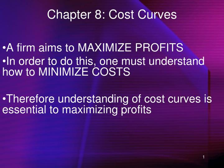
Chapter 8: Cost Curves. A firm aims to MAXIMIZE PROFITS In order to do this, one must understand how to MINIMIZE COSTS Therefore understanding of cost curves is essential to maximizing profits. Chapter 8: Costs Curves. In this chapter we will cover: 8.1 Long Run Cost Curves

E N D
Chapter 8: Cost Curves • A firm aims to MAXIMIZE PROFITS • In order to do this, one must understand how to MINIMIZE COSTS • Therefore understanding of cost curves is essential to maximizing profits
Chapter 8: Costs Curves In this chapter we will cover: 8.1 Long Run Cost Curves 8.1.1 Total Cost 8.1.2 Marginal Cost and Average Cost 8.2 Economies of Scale 8.3 Short Run Cost Curves 8.3.1 Total Cost, Variable Cost, Fixed Cost 8.3.2 Marginal Cost and Average Cost 8.4 Economies of Scope 8.5 Economies of Experience
8.1 Long Run Cost Curves • In the long run, a firm’s costs equal zero when zero production is undertaken • As production (Q) increases, the firm must use more inputs, thus increasing its cost • By minimizing costs, a firm’s long run cost curve is as follows:
K Q1 Q0 • TC = TC0 K1 • K0 TC = TC1 0 L (labor services per year) L0 L1 TC ($/yr) LR Total Cost Curve TC1=wL1+rK1 TC0 =wL0+rK0 Q (units per year) Q1 0 Q0
Input Prices and LR Cost Curves • An increase in the price of only 1 input will cause a firm to change its optimal choice of inputs • However, the increase in input costs will always cause a firm’s costs to increase: • -(This is only not true in the case of perfect substitutes when the productivity per dollar of each substitute is originally equal)
K C1: Original isocost curve (TC = $200) C2: Isocost curve after Price change (TC = $200) C3: Isocost curve after Price change (TC = $300) Slope=w1/r TC1/r A • TC0/r B • Slope=w2/r Q0 C2 C3 C1 0 L
TC ($/yr) Change in Input Prices ->A Shift in the Total Cost Curve TC(Q) new TC(Q) old 300 200 Q (units/yr) Q0
Example • Let Q=2(LK)1/2 MRTS=K/L, • W=5, R=20, Q=40 • What occurs to costs when rent falls to 5? • Initially: • MRTS=W/R • K/L=5/20 • 4K=L • Q=2(LK)1/2 • 40=2(4KK)1/2 • 40=4K • 10=K • 40=L
Example • Let Q=2(LK)1/2 MRTS=K/L, • W=5, R=20, Q=40 • What occurs to costs when rent falls to 5? • After Price Change: • MRTS=W/R • K/L=5/5 • L=K • Q=2(LK)1/2 • 40=2(LL)1/2 • 40=2L • 20=L • 20=K
What occurs when rent falls to 5? • Initial: L=40, K=10 Final: L=K=20 • W=5, R=20, Q=40 • Initial: TC=wL+rK • TC=5(40)+20(10) • TC=400 • Final: TC=5(20)+5(20) • TC=200 • Due to the fall in rent, total cost falls by $200.
TC ($/yr) Change in Rent TC(Q) initial TC(Q) final 400 200 Q (units/yr) 40
8.1.1 Total Cost • To calculate total cost, simply substitute labour and capital demand into your cost expression: • Q= 50L1/2K1/2 (From Chapter 7, slide 38:) • L*(Q,w,r) = (Q0/50)(r/w)1/2 • K*(Q,w,r) = (Q0/50)(w/r)1/2 • TC = wL +rK • TC= w [(Q0/50)(r/w)1/2 ]+r[(Q0/50)(w/r)1/2 ] • TC= [(Q0/50)(wr)1/2 ]+[(Q0/50)(wr)1/2 ] • TC = 2Q0(wr)1/2 /50
Total Cost Example 2 Let Q= L1/2K1/2, MPL/MPK=K/L, w=10, r=40. Calculate total cost. MRTS=w/r K/L=10/40 K=4L Q=L1/2K1/2 =L1/2(4L)1/2 Q=2L L=Q/2
Total Cost Example 2 Let Q= L1/2K1/2, MRTS=K/L, w=10, r=40. Calculate total cost. Q=L1/2K1/2 Q=(K/4)1/2K1/2 Q=1/2K K=2Q TC = wL +rK TC = 10(Q/2) +40(2Q) TC=85Q K=4L L=K/4 L=Q/2
Input Prices and LR Cost Curves • When the price of all inputs change by the same (percentage) amount, the optimal input combination does not change • The same combination of inputs are purchased at higher prices
K (capital services/yr) • C1=Isocost curve before ($200) and after ($220) a 10% increase in input prices A • Q0 C1 0 L (labor services/yr)
TC ($/yr) Example: A Shift in the Total Cost Curve When Input Prices Rise 10% TC(Q) new TC(Q) old 220 200 Q (units/yr) Q0
8.1.2 Average and Marginal Cost Functions • Definition: The long run average cost function is the long run total cost function divided by output, Q. • That is, the LRAC function tells us the firm’s cost per unit of output…
Long Run Average and Marginal Cost Functions • Definition: The long run marginal cost function is rate at which long run total cost changes with a change in output • The (LR)MC curve is equal to the slope of the (LR)TC curve
TC ($/yr) Average vrs. Marginal Costs TC(Q) post Slope=LRMC TC0 Slope=LRAC Q (units/yr) Q0
Relationship Between Average and Marginal Costs • When marginal cost is less than average cost, average cost is decreasingin quantity. That is, if MC(Q) < AC(Q), AC(Q) decreases in Q. • When marginal cost is greater than average cost, average cost is increasingin quantity. That is, if MC(Q) > AC(Q), AC(Q) increases in Q. • When marginal cost equals average cost, average cost does not change with quantity. That is, if MC(Q) = AC(Q), AC(Q) is flat with respect to Q.
AC, MC ($/yr) “typical” shape of AC, MC MC AC • AC at minimum when AC(Q)=MC(Q) 0 Q (units/yr)
8.2 Economies and Diseconomies of Scale • If average cost decreases as output rises, all else equal, the cost function exhibits economies of scale. • -large scale operations have an advantage • If average cost increases as output rises, all else equal, the cost function exhibits diseconomies of scale. • -small scale operations have an advantage
Economies and Diseconomies of Scale • Why Economies of scale? • -Increasing Returns to Scale for Inputs • -Specialization of Labour • -Indivisible Inputs (ie: one factory can produce up to 1000 units, so increasing output up to 1000 decreases average costs for the factory)
Economies and Diseconomies of Scale • Why Diseconomies of scale? • -Diminishing Returns from Inputs • -Managerial Diseconomies • -Growing in size requires a large expenditure on managers • -ie: One genius cannot run more than 1 branch
AC ($/yr) Typical Economies of Scale Minimum Efficient Scale – smallest Quantity where LRAC curve reaches Its min. AC(Q) Economies of scale Diseconomies of scale 0 Q (units/yr) Q*
Returns to Scale and Economies of Scale • When the production function exhibits increasing returns to scale, the long run average cost function exhibits economies of scale so that AC(Q) decreases with Q, all else equal. • When the production function exhibits decreasing returns to scale, the long run average cost function exhibits diseconomies of scale so that AC(Q) increases with Q, all else equal.
Returns to Scale and Economies of Scale • When the production function exhibits constant returns to scale, the long run average cost function is flat: it neither increases nor decreases with output. • Production Function => Returns to Scale • Costs => Economies of Scale
Example: Returns to Scale and Economies of Scale CRS IRS DRS Production Function Q = L Q = L2 Q = L1/2 Labor Demand L*=Q L*=Q1/2 L*=Q2 Total Cost Function TC=wQ wQ1/2 wQ2 Average Cost Function AC=w w/Q1/2 wQ Economies of Scale none EOS DOS
Measuring Economies of Scale - Output Elasticity of Total Cost • Economies of Scale can be measured using output elasticity of total cost; how cost changes when output changes
Measuring Economies of Scale - Output Elasticity of Total Cost • Economies of Scale are also related to marginal cost and average cost
If TC,Q < 1, MC < AC, so AC must be decreasing in Q. Therefore, we have economies of scale. • If TC,Q > 1, MC > AC, so AC must be increasing in Q. Therefore, we have diseconomies of scale. • If TC,Q = 1, MC = AC, so AC is just flat with respect to Q.
Example • Let Cost=50+20Q2 • MC=40Q • IF Q=1 or Q=2, determine economies of scale • (Let Q be thousands of units)
Example • TC=50+20Q2 • MC=40Q • AC=TC/Q=50/Q+20Q • Initially: MC=40(1)=40 • AC=50/1+20(1)=70 • Elasticity=MC/AC=40/70 – Economies of Scale • Finally: MC=40(2)=80 • AC=50/2+20(2)=65 • E=MC/AC=80/65 – Diseconomies of Scale
8.3 Short-Run Cost Curves • In the short run, at least 1 input is fixed (ie: (K=K*) • Total fixed costs (TFC) are the costs associated with this fixed input (ie: rk) • Total variable costs (TVC) are the costs associated with variable inputs (ie:wL) • Short-run total costs are fixed costs plus variable costs: STC=TFC+TVC
TC ($/yr) Short Run Total Cost, Total Variable Cost and Total Fixed Cost STC(Q, K*) TVC(Q, K*) rK* TFC rK* Q (units/yr)
Short Run Costs Example: Minimize the cost to build 80 units if Q=2(KL)1/2 and K=25. If r=10 and w=20, classify costs. Q=2(KL)1/2 80=2(25L)1/2 80=10(L)1/2 8=(L)1/2 64=L
Short Run Costs Example: K*=25, L=16. If r=10 and w=20, classify costs. TFC=rK*=10(25)=250 TVC=wL=20(64)=1280 STC=TFC+TVC=1530
Relationship Between Long Run and Short Run Total Cost Functions • The firm can minimize costs better in the long run because it is less constrained. • Hence, the short run total cost curve lies above the long run total cost curve almost everywhere.
K Only at point A is short run minimized as well as long run TC2/r Q1 Long Run Expansion path TC1/r TC0/r C • Q0 Short Run Expansion path Q0 A • • B K* 0 L TC0/w TC1/w TC2/w
TC ($/yr) STC(Q) LRTC(Q) A • rK* Q (units/yr)
8.3.2 Short Run Average and Marginal Cost Functions • Definition: The short run average cost function is the short run total cost function divided by output, Q. • That is, the SAC function tells us the firm’s cost per unit of output…
Short Run Average and Marginal Cost Functions • Definition: The short run marginal cost function is rate at which short run total cost changes with a change in input • The SMC curve is equal to the slope of the STC curve
Short Run Average and Marginal Cost Functions • In the short run, 2 additional average costs exist: average variable costs (AVC) and average fixed costs (AFC)
Example • To make an omelet, one must crack a fixed number of eggs (E) and add a variable number of other ingredients (O). Total costs for 10 omelets were $50. Each omelet’s average variable costs were $1.50. If eggs cost 50 cents, how many eggs in each omelet? • AC=AVC+AFC • TC/Q=AVC+AFC • 50/10=$1.50+AFC • $3.50=AFC
Example • To make an omelet, one must crack a fixed number of eggs (E) and add a variable number of other ingredients (O). Total costs for 10 omelets were $50. Each omelet’s average variable costs were $1.50. If eggs cost 50 cents, how many eggs in each omelet? • $3.50=AFC • $3.50=PE (E/Q) • $3.50=0.5 (E/Q) • 7=E/Q • There were 7 eggs in each omelet.
$ Per Unit Average fixed cost is constantly decreasing, as fixed costs don’t rise with output. AFC 0 Q (units per year)
$ Per Unit Average variable cost generally decreases then increases due to economies of scale. AVC AFC 0 Q (units per year)
SAC is the vertical sum of AVC and AFC $ Per Unit SAC AVC Equal AFC 0 Q (units per year)