Download
1 / 26
260 likes | 372 Vues
J. Feigenbaum, S. Kannan, J. Zhang. Computing Diameter in the Streaming and Sliding-Window Models. Introduction. Two computational models: Streaming model Sliding-window model

E N D
J. Feigenbaum, S. Kannan, J. Zhang Computing Diameter in the Streaming and Sliding-Window Models
Introduction • Two computational models: • Streaming model • Sliding-window model • The problem: diameter of a point set P in R2. The diameter is the maximum pairwise distance between points in P.
More about Models The streaming model • A data stream is a sequence of data elements a1a2 , ..., am. • A streaming algorithm is an algorithm that computes some function over a data stream and has the following properties: • The input data are accessed in a sequential order. • The order of the data elements in the stream is not controlled by the algorithm • The length of the stream, m, is huge. Only space-efficient algorithms (sublinear or even polylog(m)) are considered.
Dynamic Algorithm in Computational Geometry • Dynamic means that the set of objects under consideration may change. There could be additions and deletions to the point set P. • Maintain the current set of geometry objects in certain data structures. Efficient updating and query answering are emphasized. • May use linear space ─ different from the requirement of the streaming and the sliding-window models.
More about Models (Continued) The sliding-window model • The inputis still a stream of data elements. • A data element arrives at each time instant; it later expires after a number of time stamps equal to the window sizen • The current window at any time instant is the set of data elements that have not yet expired.
Computing Diameter in the Streaming Model • A well-known diameter-approximation is streaming in nature. • Project the points onto lines. • Requires θ ≤ such that |π(p)π(q)|≥|pq| cosθ ≥(1− θ2/2)|pq|≥ (1−ε)|pq| • The algorithm goes through the input once. It needs storage for O(1/ ) points. To process each point, it performs O(1/ ) projections.
Diameter Approximation in the Streaming Model Theorem 1There is a streaming ε-approximation algorithm for diameter that needs storage for O(1/ε) points and processes each point in O(log(1/ε)) time. • Take the first point of the stream as the “center” and divide the space into sectors of angle θ = ε/2(1-ε). • For each sector, keep the point furthest from the center in that sector.
Diameter Approximation in the Streaming Model Let H be the maximum distance between the center and any other point and Ti,j be the minimal distance between the boundary arcs of sector i (bb') and sector j (aa'). Approximate the diameter with max{H, maxi,j Tij}
Maintaining Diameter in the Sliding-Window Model • Our space efficient mehtod maintains the diameter for sliding windows when the set of points P can be bounded in a box that is not too “large”. • Let R be the maximum, over all windows, the ratio of the diameter over the minimal non-zero distance between any two points in that window. • That the bounding space is “not too large” means R < 2n.
Maintaining Diameter in the Sliding-Window Model Theorem 2There is an ε-approximation algorithm that maintains the diameter for a planar point set in the sliding-window model using Poly(1/ε, log n, log R) bits of space.
Remove Irrelevant Points • Consider maintaining the diameter in 1-d. • A point will never realize any diameter if it is spatially located between two newer points. • Remove these points. The locations of the remaining points would look like: (where a1 is newer than a2 which is newer than a3...) • The newer points would be located “inside” and the older points would be located “outside”
The “Rounding” Method • Take the newest point as the “center,” and “round” down other points. • Divide the line into the following intervals such that |cti| = ( 1+ε )id for some distance d (to be specified later). • Round all points in the interval [ti, ti+1) down to ti. • In what follows we call the set of pints after “rounding” a cluster. If 2i original points are grouped into a cluster, we say the cluster is at level i.
Number of Points in a Cluster • If multiple points are rounded to the same location, we can discard the older ones and only keep the newest one. • In each interval, we have only one point. Let D be the diameter, the number of points k in a cluster is bounded by: k≤ log1+εD/d = (log D/d)/log (1+ε) ≤ (2/ε )log D/d
When Window Starts Sliding • Need to consider addition and deletion. • Deletion is easy, because the oldest point must be one of the cluster's extreme points. • Addition is complicated, because we may need to update the cluster center for each point that arrives. • Our solution: keep multiple clusters.
Multiple Clusters in a Window • We allow at most two clusters to be at each “level”. • When the number of clusters of “level” i exceeds 2, merge the oldest twe clusters to form a “cluster” at “level” i+1. • The window can thus be divided into clusters.
Merge Clusters • Cluster c1+cluster c2 = cluster c3 • Make Ctr2 the center of cluster c3
Merge Clusters (Continued) • Discard the points in c1 that are located between the centers of c1 and c2. • If point p in c1 satisfies |pCtr1| ≤ (1+ε)|Ctr1Ctr2|, discard it, too.
Merge Clusters (Continued) • Round the points in c2 and those remaining in c1 after the previous two steps using the center Ctr2. • The value for d is lower bounded by ε ∙ |Ctr1Ctr2|. The number of points in a cluster is then bounded by: (2/ε )(log R + log1/ε )
The Algorithm in 1-d • Update: when a new point arrives, • Check the age of the boundary points of the oldest cluster. If one of them has expired, remove it. • Make the newly arrived point a cluster of size 1. Go through the clusters and merge clusters whenever necessary according to the rules stated above. • While going throught the clusters, update the boundary points of any cluster changed. • Update the window boundary points if necessary. • Query Answer: Report the distance between the window boundary points as the window diameter.
Space Requirement • Let diamp be a diameter realized by point p. Each time we do “rounding,” we introduce a displacement for p at most ε ∙diamp. Also p can be “rounded” at most log n times. • Choose ε to be at most ε/(2log n) to bound the error. • There are at most 2log n clusters and in each cluster at most O(1/ε log n (log R + log log n + log 1/ε )) points. Keeping the age may require log n space for each point. The total space required is: O(1/ε log3n (log R + log log n + log 1/ε ))
Time Complexity • Query answer time is O(1). • Worst case update time is O(1/ε log2n (log R + log log n + log 1/ε )) because we may have cascading merges. • The amortized update time is O(log n)
Extend the Algorithm to 2-d • We will have a set of lines l0, l1, ... and project the points in the plane onto the lines. • Guarantee that any paire of points will be projected to a line with angle φ such that 1− cos φ ≤ ε/2 • Use the diameter-maintenance algorithm in 1-d for each line. • Everything will have a multiplicative overhead of O(1/ ).
Lower Bound for Maintaining Exact Diameter Theorem 3To maintain the exact diameter in a sliding window model requiresΩ(n) bits of space. Consider 2n points {a1, a2, ..., a2n} with the following properties: • an+1, an+2, ..., a2n are located at coordinate zero. • |a1an| ≥ |a2an+1| ≥ |a3an+2| ≥ ... ≥ |an-1a2n-2| = 1 • The coordinates of the points aj for j = 1,2,..., n-2 have the form n∙k for some k = 1,2,..., n.
an an+1 an+2 ...... an-1 a2 a1 an-2 A Family of Point Sequences We show below two sequences in the family: an an+1 an+2 ...... an-1 a2 a1 an-2 ......
Lower Bound for Maintaining Exact Diameter (Countinued) • There are at least different sequences of 2npoints satisfying the above properties. • Need O(n) space to distinguish them. (Note here R ≤n2 << 2n)