Download
1 / 10
110 likes | 297 Vues
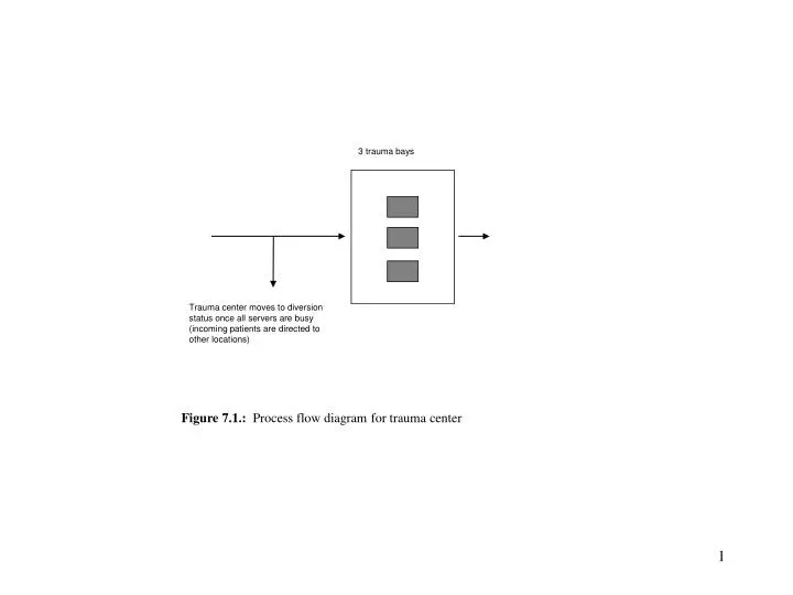
3 trauma bays. Trauma center moves to diversion status once all servers are busy (incoming patients are directed to other locations). Figure 7.1.: Process flow diagram for trauma center. Given P m (r) we can compute: Time per day that system has to deny access

E N D
3 trauma bays Trauma center moves to diversion status once all servers are busy (incoming patients are directed to other locations) Figure 7.1.: Process flow diagram for trauma center
Given Pm(r) we can compute: • Time per day that system has to deny access • Flow units lost = 1/a * Pm (r) Analyzing Loss Systems: Finding Pm(r) m • Define r = p / a • Example: r= 2 hours/ 3 hours r=0.67 • Recall m=3 • Use Erlang Loss Table • Find that P3 (0.67)=0.0255 r = p / a
Erlang Loss Table Probability{all m servers busy}=
0.6 Probabilitythat all serversare utilized 0.5 0.4 m=1 m=2 0.3 0.2 m=3 m=5 m=10 0.1 m=20 0 0 0.1 0.2 0.3 0.4 0.5 0.6 0.7 0.8 0.9 1 1.1 Implied utilization Figure 7.2.: Implied utilization vs probability of having all servers utilized
Probabilitythat system isfull, Pm Percentageof demand rate 100 0.5 80 0.4 Increasing levels of utilization 60 0.3 Increasing levels of utilization 40 0.2 20 0.1 0 0 1 2 3 4 5 6 7 8 9 10 11 1 2 3 4 5 6 7 8 9 10 11 Size of the buffer space Size of the buffer space Figure 7.3: Impact of buffer size on the probability Pm for various levels of implied utilization as well as on the throughput of the process in the case of one single server
Fraction of customer lost Average wait time [seconds] Figure 7.4.: Impact of waiting time on customer loss
Outflow of resource 1 = Inflow of resource 2 Inflow Outflow Upstream Downstream Figure 7.5.: A serial queuing system with three resources
Resource is blocked Activity completed Inflow Outflow Outflow Inflow Activity not yet completed Resource is starved Empty space for a flow unit Space for a flow unit with a flow unitin the space Figure 7.6.: The concepts of blocking and starving
6.5 min/unit 6.5 min/unit 6.5 min/unit 7 min/unit 7 min/unit 7 min/unit 6 min/unit 6 min/unit 6 min/unit Sequential system, no buffers Cycle time=11.5 minutes Sequential system, unlimited buffers Cycle time=7 minutes; inventory “explodes” 3 resources, 19.5 min/ unit each (1) (1) Horizontally pooled system Cycle time=19.5/3 minutes=6.5 minutes Sequential system, one buffer space each Cycle time=10 minutes Figure 7.7.: Flow rate compared at four configurations of a queuing system
Waitingproblem Loss problem Pure waitingproblem, all customersare perfectly patient. All customers enter the process,some leave due totheir impatience Customers do notenter the process oncebuffer has reached a certain limit Customers are lostonce all servers arebusy Same if customers are patient Same if buffer size=0 Same if buffer size is extremely large Figure 7.8.: Different types of variability problems