Download

1 / 55
630 likes | 1.13k Vues
Quantization. Does the digital representation of an analog value have anything to do with the digital filtering process?.

E N D
Does the digital representation of an analog value have anything to do with the digital filtering process? Digital representations of analog signals are in the form of bits. These bits are taken from an analog-to-digital converter, processed and then put to a digital-to-analog converter. bits x y A/D Filtering D/A bits
Up until this point we have been dealing with sampled analog functions, where each sample is represented by a real number. A real number cannot be represented with complete accuracy. The samples are represented (in a computer) by a finite number of bits representing the number as an integer or a floating-point number. We determined the number of samples per second that was needed to accurately represent the analog signal. We will now consider the number of bits needed per sample to accurately represent the analog signal.
WithB bits, we can represent 2B different values. For example, if B=3, we can have eight different values corresponding to 000, 001, 010, 011, 100, 101, 110, 111. The 2B values can correspond to volts, millivolts, multiplies of 0.25 volts, etc.
Example: Suppose we had B=3 bits corresponding to a number which is equal to the voltage of a signal (at some point in time). The 23=8 different voltage levels are 0V, 1V, 2V, 3V, 4V, 5V, 6V and 7V. A digital-to-analog converter would convert 000 to 0V, 001 to 1V, etc. An analog-to-digital converter would convert an input signal at 0V to 000. An input of 1V would be converted to 001; an input of 2V would be converted to 010, etc.
Suppose the input signal to an analog-to-digital converter were 1.5V. Would this voltage be converted to 001 or 010? The answer depends upon the type of quantization used by the analog-to-digital converter. If the type of quantization is truncation, then allvalues from 1.0V up to but not including 2.0V are converted to 001. If the type of quantization is rounding, then allvalues from 0.5V up to but not including 1.5V are converted to 001. Values of from 1.5V up to but not including 2.5V are converted to 010.
^ Let xbe the quantized version of x. While x can take on any value, x can only take on discrete values corresponding to the output of a digital-to-analog converter such as 1.0, 2.0, 3.0 (volts). ^ If we cascade an analog-to-digital converter with a digital-to-analog converter we will get a quantizer that converts x to x. ^ 000, 001, … ^ x x A/D D/A
^ The relationships between x and x are shown on the following graphs.
^ x Truncation 111 7 110 6 101 5 100 4 011 3 010 2 001 1 000 x 1 2 3 4 5 6 7 8
^ x Rounding 7 6 5 4 3 2 1 x 1 2 3 4 5 6 7 8
Negative values can also be represented digitally. There are two common formats: sign magnitude and two’s complement. In sign magnitude format, the most significant bit is a sign bit:1 is negative,0 is positive. In two’s complement format, positive numbers are like normal positive numbers. Negative numbers are wrapped backwards: -1 is 111, -2 is 110, etc.
Shown on the following graphs are signed quantization levels and values for truncation and rounding quantization, and sign magnitude and two’s complement formats.
^ x Truncation, Sign Magnitude 011 010 001 x 000 101 110 111
^ x Truncation, Two’s Complement 011 010 001 x 000 111 110 101 100
^ x Rounding, Sign Magnitude 011 010 001 x 000 101 110 111
^ x Rounding, Two’s Complement 011 010 001 x 000 111 110 101 100
In all of the previous quantization examples, the step size was one (1). The step size could be 0.5, 0.25, etc. Let D be the step size, also known as the quantization interval. For truncation quantization, the quantization error is between 0 and D. For rounding quantization, the quantization error is between -D/2 and +D/2.
The ratio of the maximum signal magnitude to the quantization interval is a measure of the fidelity of the digitized sample. Let us see if we can relate this ratio to a more common ratio called the signal-to-noise ratio (SNR). Let A be the maximum magnitude of a signal. The ratio of the maximum magnitude to the quantization interval is A/D. The signal-to-noise ratio is a ratio of powers. The power in a signal is related to its distribution.
If the signal is uniformlydistributed between –A and A, the distribution looks like this: px(x) x -A A
In many cases, we can assume that the distribution of the quantization error, e, is uniform: pe(e) Truncation e D
In many cases, we can assume that the distribution of the quantization error, e, is uniform: pe(e) Rounding e -D/2 D/2
The power may be obtained from a distribution by integrating the product of the distribution with x2 or e2.
We can now calculate the signal-to-noise ratio for a uniformly distributed signal with truncation and rounding quantization:
Exercise: If we use B-bit quantization (with 2B quantization levels), express the signal-to-noise ratio in dB [=10 log (power ratio)] in terms of Bfor both truncation and rounding quantization. (In both cases, 2A/D = 2B.)
Error or distortion due to quantization has an effect on the signal. Quantization error also has an effect on the filtering process.
Example: Consider the following filter (transfer function): Suppose we apply a pulse x[n]=d[n] to this filter. The expected response is y[n] = (0.75)n.
Now suppose we introduce quantization into the arithmetic. Let B=3, or q=1/8. The result is as follows:
The quantized output does not go to zero: it levels-off at a final value of y[n] = 0.25. The resultant “leveling-off” effect is called the deadband effect. The result gets even worse as the poles get close to the unit circle. Suppose we modified the previous example to change the location of the pole from z=0.75 to z=0.875.
The results for the impulse response are shown on the following slides in tabular and graphic form.
Exercise: Find the impulse response to the following filter: Use three-bit quantization, then try four-bit quantization.
Let us generalize this quantization problem in filtering. In our previous examples we had a filter function of the form
The corresponding difference equation is This operation needs to be performed for each input sample (and output sample). The quantization error occurs in the multiplication of a and y[n-1].
Since this error occurs for each sample, the error is compounded by repeated calculations. To see the final, net effect of this error, let us look at the final, steady-state value of ŷ[n] which we will denote by ŷf
For rounding truncation, So, the net error would have the following range:
This idea can be extended to a general filter expressed as a polynomial fraction: We will have
Example: Use the derived relationship on the bounds of the final error for each of the following filters:
The net error due to quantization and filtering is also dependent upon the order and manner in which the filter operations are performed. As an example, consider the following filter
We can also implement this filter as The corresponding difference equation is
We can also implement this filter as This can be thought of as a compoundfilter: