Download
1 / 37
380 likes | 610 Vues
EECS 122: Introduction to Computer Networks Link State and Distance Vector Routing. Computer Science Division Department of Electrical Engineering and Computer Sciences University of California, Berkeley Berkeley, CA 94720-1776. Today’s Lecture: 7. 2. 17, 18, 19. Application. 10, 11. 6.

E N D
EECS 122: Introduction to Computer Networks Link State and Distance Vector Routing Computer Science Division Department of Electrical Engineering and Computer Sciences University of California, Berkeley Berkeley, CA 94720-1776
Today’s Lecture: 7 2 17, 18, 19 Application 10, 11 6 Transport 14, 15, 16 7, 8, 9 Network (IP) 21, 22, 23 Link Physical 25
IP Header • Vers: IP versions • HL: Header length (in 32-bits) • Type: Type of service • Length: size of datagram (header + data; in bytes) • Identification: fragment ID • Fragment offset: offset of current fragment (x 8 bytes) • TTL: number of network hops • Protocol: protocol type (e.g., TCP, UDP) • Source IP addresses • Destination IP address
What is Routing? Routing is the core function of a network It ensures that • information accepted for transfer • at a source node • is delivered to the correct • set of destination nodes, • at reasonable levels of performance.
Internet Routing • Internet organized as a two level hierarchy • First level – autonomous systems (AS’s) • AS – region of network under a single administrative domain • AS’s run an intra-domain routing protocols • Distance Vector, e.g., Routing Information Protocol (RIP) • Link State, e.g., Open Shortest Path First (OSPF) • Between AS’s runs inter-domain routing protocols, e.g., Border Gateway Routing (BGP) • De facto standard today, BGP-4
Example Interior router BGP router AS-1 AS-3 AS-2
Intra-domain Routing Protocols • Based on unreliable datagram delivery • Distance vector • Routing Information Protocol (RIP), based on Bellman-Ford • Each neighbor periodically exchange reachability information to its neighbors • Minimal communication overhead, but it takes long to converge, i.e., in proportion to the maximum path length • Link state • Open Shortest Path First (OSPF), based on Dijkstra • Each network periodically floods immediate reachability information to other routers • Fast convergence, but high communication and computation overhead
5 3 5 2 2 1 3 1 2 1 C D B A E F Routing • Goal: determine a “good” path through the network from source to destination • Good means usually the shortest path • Network modeled as a graph • Routers nodes • Link edges • Edge cost: delay, congestion level,…
Outline • Link State • Distance Vector
Dijkstra’s algorithm Net topology, link costs known to all nodes Accomplished via “link state flooding” All nodes have same info Compute least cost paths from one node (‘source”) to all other nodes Iterative: after k iterations, know least cost paths to k closest destinations Notations c(i,j): link cost from node i to j; cost infinite if not direct neighbors D(v): current value of cost of path from source to destination v p(v): predecessor node along path from source to v, that is next to v S: set of nodes whose least cost path definitively known A Link State Routing Algorithm
Link State Flooding Example 5 7 4 8 6 11 2 10 3 1 13 12
Link State Flooding Example 5 7 4 8 6 11 2 10 3 1 13 12
Link State Flooding Example 5 7 4 8 6 11 2 10 3 1 13 12
Link State Flooding Example 5 7 4 8 6 11 2 10 3 1 13 12
Dijsktra’s Algorithm 1 Initialization: 2 S = {A}; 3 for all nodes v 4 if v adjacent to A 5 then D(v) = c(A,v); 6 else D(v) = ; 7 8 Loop 9 find w not in S such that D(w) is a minimum; 10 add w to S; 11 update D(v) for all v adjacent to w and not in S: 12 D(v) = min( D(v), D(w) + c(w,v) ); // new cost to v is either old cost to v or known // shortest path cost to w plus cost from w to v 13 until all nodes in S;
C D E A B F Example: Dijkstra’s Algorithm D(B),p(B) 2,A D(D),p(D) 1,A D(C),p(C) 5,A D(E),p(E) Step 0 1 2 3 4 5 start S A D(F),p(F) 1 Initialization: 2 S = {A}; 3 for all nodes v 4 if v adjacent to A 5 then D(v) = c(A,v); 6 else D(v) = ; … 5 3 5 2 2 1 3 1 2 1
C D E A B F Example: Dijkstra’s Algorithm D(B),p(B) 2,A D(D),p(D) 1,A D(C),p(C) 5,A 4,D D(E),p(E) 2,D Step 0 1 2 3 4 5 start S A AD D(F),p(F) • … • 8 Loop • 9 find w not in S s.t. D(w) is a minimum; • 10 add w to S; • update D(v) for all v adjacent • to w and not in S: • 12 D(v) = min( D(v), D(w) + c(w,v) ); • 13 until all nodes in S; 5 3 5 2 2 1 3 1 2 1
C D E A B F Example: Dijkstra’s Algorithm D(B),p(B) 2,A D(D),p(D) 1,A D(C),p(C) 5,A 4,D 3,E D(E),p(E) 2,D Step 0 1 2 3 4 5 start S A AD ADE D(F),p(F) 4,E • … • 8 Loop • 9 find w not in S s.t. D(w) is a minimum; • 10 add w to S; • update D(v) for all v adjacent • to w and not in S: • 12 D(v) = min( D(v), D(w) + c(w,v) ); • 13 until all nodes in S; 5 3 5 2 2 1 3 1 2 1
C D E A B F Example: Dijkstra’s Algorithm D(B),p(B) 2,A D(D),p(D) 1,A D(C),p(C) 5,A 4,D 3,E D(E),p(E) 2,D Step 0 1 2 3 4 5 start S A AD ADE ADEB D(F),p(F) 4,E • … • 8 Loop • 9 find w not in S s.t. D(w) is a minimum; • 10 add w to S; • update D(v) for all v adjacent • to w and not in S: • 12 D(v) = min( D(v), D(w) + c(w,v) ); • 13 until all nodes in S; 5 3 5 2 2 1 3 1 2 1
C D E A B F Example: Dijkstra’s Algorithm D(B),p(B) 2,A D(D),p(D) 1,A D(C),p(C) 5,A 4,D 3,E D(E),p(E) 2,D Step 0 1 2 3 4 5 start S A AD ADE ADEB ADEBC D(F),p(F) 4,E • … • 8 Loop • 9 find w not in S s.t. D(w) is a minimum; • 10 add w to S; • update D(v) for all v adjacent • to w and not in S: • 12 D(v) = min( D(v), D(w) + c(w,v) ); • 13 until all nodes in S; 5 3 5 2 2 1 3 1 2 1
C D E A B F Example: Dijkstra’s Algorithm D(B),p(B) 2,A D(D),p(D) 1,A D(C),p(C) 5,A 4,D 3,E D(E),p(E) 2,D Step 0 1 2 3 4 5 start S A AD ADE ADEB ADEBC ADEBCF D(F),p(F) 4,E • … • 8 Loop • 9 find w not in S s.t. D(w) is a minimum; • 10 add w to S; • update D(v) for all v adjacent • to w and not in S: • 12 D(v) = min( D(v), D(w) + c(w,v) ); • 13 until all nodes in S; 5 3 5 2 2 1 3 1 2 1
Complexity • Assume a network consisting of n nodes • Each iteration: need to check all nodes, w, not in S • n*(n+1)/2 comparisons: O(n2) • More efficient implementations possible: O(n*log(n))
e C C C C D D D D A A B A B B B A 0 2+e 2+e 2+e 0 0 0 0 1 1 1+e 1+e 1 1+e 0 e 0 0 … recompute … recompute routing … recompute Oscillations • Assume link cost = amount of carried traffic 1 1+e 0 0 e 0 1 1 initially • How can you avoid oscillations?
Outline • Link State • Distance Vector
Distance Vector Routing Algorithm • Iterative: continues until no nodes exchange info • Asynchronous: nodes need not exchange info/iterate in lock steps • Distributed: each node communicates only with directly-attached neighbors • Each router maintains • Row for each possible destination • Column for each directly-attached neighbor to node • Entry in row Y and column Z of node X best known distance from X to Y, via Z as next hop (remember this !) • Note: for simplicity in this lecture examples we show only the shortest distances to each destination
wait for (change in local link cost or msg from neighbor) recompute distance table if least cost path to any dest has changed, notify neighbors Distance Vector Routing Each node: • Each local iteration caused by: • Local link cost change • Message from neighbor: its least cost path change from neighbor to destination • Each node notifies neighbors only when its least cost path to any destination changes • Neighbors then notify their neighbors if necessary
Distance Vector Algorithm (cont’d) • 1 Initialization: • 2 for all neighbors V do • 3 ifV adjacent to A • 4 D(A, V) = c(A,V); • 5 else • D(A, V) = ∞; • loop: • 8 wait (until A sees a link cost change to neighbor V • 9 or until A receives update from neighbor V) • 10 if (D(A,V) changes by d) • 11 for all destinations Y through Vdo • 12 D(A,Y) = D(A,Y) + d • 13 else if (update D(V, Y) received from V) • /* shortest path from V to some Y has changed */ • 14 D(A,Y) = D(A,V) + D(V, Y); • 15 if (there is a new minimum for destination Y) • 16 send D(A, Y) to all neighbors • 17 forever
C D B A Example: Distance Vector Algorithm Node A Node B 3 2 1 1 7 Node C Node D • 1 Initialization: • 2 for all neighbors V do • 3 ifV adjacent to A • 4 D(A, V) = c(A,V); • else • D(A, V) = ∞; • …
D C B A Example: 1st Iteration (C A) Node A Node B 3 2 1 1 7 D(A, D) = D(A, C) + D(C,D) = 7 + 1 = 8 (D(C,A), D(C,B), D(C,D)) Node C Node D • loop: • … • 13 else if (update D(V, Y) received from V) • 14 D(A,Y) = D(A,V) + D(V, Y); • 15 if (there is a new min. for destination Y) • 16 send D(A, Y) to all neighbors • 17 forever
D C B A Example: 1st Iteration (BA, CA) Node A Node B 3 2 1 1 7 D(A,D) = D(A,B) + D(B,D) = 2 + 3 = 5 D(A,C) = D(A,B) + D(B,C) = 2 + 1 = 3 Node C Node D • loop: • … • 13 else if (update D(V, Y) received from V) • 14 D(A,Y) = min(D(A,V), D(A,V) + D(V, Y)) • 15 if (there is a new min. for destination Y) • 16 send D(A, Y) to all neighbors • 17 forever
C D B A Example: End of 1st Iteration Node A Node B 3 2 1 1 7 Node C Node D • loop: • … • 13 else if (update D(V, Y) received from V) • 14 D(A,Y) = D(A,V) + D(V, Y); • 15 if (there is a new min. for destination Y) • 16 send D(A, Y) to all neighbors • 17 forever
C D B A Example: End of 2nd Iteration Node A Node B 3 2 1 1 7 Node C Node D • loop: • … • 13 else if (update D(V, Y) received from V) • 14 D(A,Y) = D(A,V) + D(V, Y); • 15 if (there is a new min. for destination Y) • 16 send D(A, Y) to all neighbors • 17 forever
C D B A Example: End of 3rd Iteration Node A Node B 3 2 1 1 7 Node C Node D • loop: • … • 13 else if (update D(V, Y) received from V) • 14 D(A,Y) = D(A,V) + D(V, Y); • 15 if (there is a new min. for destination Y) • 16 send D(A, Y) to all neighbors • 17 forever Nothing changes algorithm terminates
1 4 1 50 C A B Distance Vector: Link Cost Changes 7 loop: 8 wait (until A sees a link cost change to neighbor V 9 or until A receives update from neighbor V) 10 if (D(A,V) changes by d) 11 for all destinations Y through Vdo 12 D(A,Y) = D(A,Y) + d 13 else if (update D(V, Y) received from V) 14 D(A,Y) = D(A,V) + D(V, Y); 15 if (there is a new minimum for destination Y) 16 send D(A, Y) to all neighbors 17 forever Node B “good news travels fast” Node C time Link cost changes here Algorithm terminates
60 4 1 50 C A B Distance Vector: Count to Infinity Problem 7 loop: 8 wait (until A sees a link cost change to neighbor V 9 or until A receives update from neighbor V) 10 if (D(A,V) changes by d) 11 for all destinations Y through Vdo 12 D(A,Y) = D(A,Y) + d ; 13 else if (update D(V, Y) received from V) 14 D(A,Y) = D(A,V) + D(V, Y); 15 if (there is a new minimum for destination Y) 16 send D(A, Y) to all neighbors 17 forever Node B “bad news travels slowly” Node C … time Link cost changes here; recall from slide 24 that B also maintains shortest distance to A through C, which is 6. Thus D(B, A) becomes 6 !
60 4 1 50 C A B Distance Vector: Poisoned Reverse • If C routes through B to get to A: • C tells B its (C’s) distance to A is infinite (so B won’t route to A via C) • Will this completely solve count to infinity problem? Node B Node C time Link cost changes here; B updates D(B, A) = 60 as C has advertised D(C, A) = ∞ Algorithm terminates
Per node message complexity LS: O(n*e) messages; n – number of nodes; e – number of edges DV: O(d) messages; where d is node’s degree Complexity LS: O(n2) with O(n*e) messages DV: convergence time varies may be routing loops count-to-infinity problem Robustness: what happens if router malfunctions? LS: node can advertise incorrect link cost each node computes only its own table DV: node can advertise incorrect path cost each node’s table used by others; error propagate through network Link State vs. Distance Vector