Download
1 / 28
300 likes | 478 Vues
Gravity wave drag Parameterization of orographic related momentum fluxes in a numerical weather processing model Andrew Orr anmcr@bas.ac.uk. Lecture 1: Atmospheric processes associated with orography. Lecture 2: Parameterization of subgrid-scale orography.

E N D
Gravity wave drag Parameterization of orographic related momentum fluxes in a numerical weather processing model Andrew Orr anmcr@bas.ac.uk Lecture 1: Atmospheric processes associated with orography Lecture 2: Parameterization of subgrid-scale orography
Equation of horizontal hydrostatic motion (linearise around mean state) Drag effects acceleration through tendencies of the horizontal wind Dyn: dynamics (resolved), e.g. advection, pressure gradient and Coriolis force Param: physical parameterizations of sub-grid scale processes: e.g. radiation, convection, boundary layer, orography (Note a prime denotes sub-grid scale deviation and an overline denotes gridbox average) Parameterized tendency related to the vertical divergence of sub-grid scale vertical momentum flux (N/m2) (also called stress) Tendency’s due to sub-grid scale orography (SSO) Equation for resolved part of the horizontal momentum
Specification of sub-grid orography h: mean (resolved) topographic height at each gridpoint * * * * x From Baines and Palmer (1990) h: topographic height above sea level (from global 1km data set) At each gridpoint sub-grid orography represented by: μ: standard deviation of h (amplitude of sub-grid orography) 2μ approximates the physical envelope of the peaks γ: anisotropy (measure of how elongated sub-grid orography is) θ: angle between x-axis and principal axis (i.e. direction of maximum slope) ψ: angle between low-level wind and principal axis of the topography σ: mean slope (along principal axis) Note source grid is filtered to remove small-scale orographic structures and scales resolved by model – otherwise parameterization may simulate unrelated effects Additional filtering so that only forced at scales the model can represent well
Evaluation of required parameters Diagonalise Direction of maximum mean-square gradient at an angle θ to the x-axis Calculate topographic gradient correlation tensor
Anisotropy defined as (1:circular; 0: ridge) Slope (i.e. mean-square gradient along the principal axis) If the low-level wind is directed at an angle φ to the x-axis, then the angle ψ is given by: Change coordinates (orientated along principal axis) (ψ=0 flow normal to obstacle; ψ=π/2 flow parallel to obstacle)
Illustration of anisotropy and principle axis of sub-grid scale orography for a number of general-circulation model grid cells near the Tibetan plateau. Contours show the unresolved orography From Scinocca and McFarlane 2000
Resolution sensitivity of sub-grid fields mean orography / land sea mask slope (σ) standard deviation (μ) Horizontal resolution: ERA40~120km; T511~40km; T799~25km
mean orography (UK Met Office Unified Model) From Smith et al. (2006)
Lott and Miller (1997) parametrization scheme heff zblk h hz/zblk Contributions from (a) gravity wave drag and (b) low-level blocking drag (a) Gravity wave drag 1. Compute gravity wave surface stress exerted on sub-grid scale orography 2. Compute vertical distribution of wave stress accompanying the surface value (b) Blocked flow drag See Lott and Miller (1997) 1. Compute depth of blocked layer 2. Compute drag at each model level for z < zblk
Compute gravity wave surface stress • Determine where and how strongly waves are excited • More, generally where is the amplitude of the displacement of the isentropic surface Effects of anisotropy on gravity wave surface stress Assume sub-grid scale orography has elliptical shape Gravity wave stress can be written as (Phillips 1984) G (~1): constant (tunes amplitude of waves) Increasing this increases gravity wave surface stress Typically L2/4ab ellipsoidal hills inside a grid point. Summing all forces we find the stress per unit area (using a=μ/σ) See Lott and Miller 1997
Compute vertical distribution of stress • Determine how strongly the waves are dissipated • Strongest dissipation occurs in regions where the wave becomes unstable and breaks down into turbulence, referred to as wave breaking • Convective instability: where the amplitude of the wave becomes so large that it causes relatively cold air to rise over less dense, warm air • Kelvin-Helmholtz instability also important: associated with shear zones • Lindzen’s saturation hypothesis: instability brings about turbulent dissipation of the wave such that the amplitude of the wave is reduced until it becomes stable again (Lindzen 1981), i.e. λequals the local saturated stress λsat • i.e. dissipation is just sufficient to ensure that • Which gives , i.e. strong dependence on U which shows that wave breaking is strong preferred in regions of weak flow. Similarly, the stronger/smaller N/ρ the more readily waves break (Palmer et al. 1986)
:amplitude of wave :mean Richardson number Saturation hypothesis in terms of Ri • Can show that wave’s impact on static stability and vertical shear gives rise to a minimum Richardson number (Palmer et al. 1986) • Instability occurs when Rimin < Ricrit (=0.25) (i.e. less than the critical value) • Kelvin-Helmholtz: numerator becomes small • Convective instability: denominator becomes large • Following saturation hypothesis, when the wave is saturated Rimin=0.25 and δh=δhsat • Wave breaking occurs more readily in this formulation than in a purely convective overturning scheme
Gravity wave breaking only active above zblk (i.e. λ=λs for 0<z< zblk) Above zblk stress constant until waves break, i.e. saturation hypothesis (Lindzen 1981) when stress exceeds saturation stress Excess stress dissipated → drag This occurs when the local Richardson number Rimin < Ricrit(=0.25). Ricrit can be used as a tuning parameter. Increasing it makes it easier for waves to break, so drag momentum deposition occurs at a lower altitude. zblk λ • Some rough figures based on a surface flux of 0.1 N m-2 (Palmer et al. 1986 This will saturate in the • Boundary layer if U< 5 m/s (preferred region of wave breaking) • Mid troposphere if U< 7 m/s (mid-troposphere winds generally like this) • Lower stratosphere if U < 15 m/s (preferred region of wave breaking)
Assume stress at any level: Calculate Ri at next level λk-2 Set λk-1=λk to estimate δh using Uk-2,Tk-2 λk-1 Repeat Uk-1,Tk-1 Calculate Rimin zk=zblk; λk= λs If Rimin<Ricrit set Rimin=Ricrit estimate h=hsat Estimate λ= λsat go to next level Height z=0; λ= λs set λk-1= λk go to next level Values of the wave stress are defined progressively from zblk upwards Set λ=λs and Rimin=0.25 at model level representing top of blocked layer If Rimin>=Ricrit
Compute depth of blocked layer Blocking height zblk satisfies: (assume h=2μ) Characterise incident flow passing over the mountain top by ρH, UH, NH (averaged between μ and 2μ) Hncrit≈1 tunes the depth of the blocked layer. If Hncrit is increased then Zblk decreases Up calculated by resolving the wind U in the direction of UH
Compute blocked-flow drag For z<zblk flow streamlines divide around mountain Drag exerted by the obstacle on the flow at these levels can be written as l(z): horizontal width of the obstacle as seen by the flow at an upstream height z (assumes each layer below zblk is raised by a factor H/zblk, i.e. reduction of obstacle width) Cd (~1): form drag coefficient (proportional to ψ) Summing over number of consecutive ridges in a grid point gives the drag r: aspect ratio of the obstacle as seen by the incident flow; B,C: constants this equation is applied quasi-implicitly level by level below zblk Consider again an elliptical mountain
Parameterized surface stresses From ECMWF T511 operational model winter summer
Resolved/parameterized drag contributions From Lott and Miller 1997 Large parameterized drag (makes up difference between resolved and measured drag) resolved drag measured drag T213 forecasts: ECMWF model with mean orography and the subgrid scale orographic drag scheme. Explicit model pressure drag and parameterized mountain drag during PYREX.
Results from Canadian Climate model of northern hemisphere winter, showing westerly gravity wave drag (tendency in m/s/d)
Impact of scheme Alleviation of systematic westerly bias Icelandic/Aleutian lows are too deep Siberian high too weak and too far south Flow too zonal / westerly bias Azores anticyclone too far east Without GWD scheme With GWD scheme Mean January sea level pressure (mb) for years 1984 to 1986 alleviation of westerly bias Analysis (best guess) better agreement From Palmer et al. 1986
Zonal mean cross-sections of zonal wind (ms-1) and temperature (K, dashed lines) for January 1984 and (a) without GWD scheme and (b) analysis Without GWD scheme cold bias westerly bias less impact in southern-hemisphere Analysis (best guess) From Palmer et al. 1986
Sensitivity of resolved orographic drag to model resolution Flow-over case Flow-blocking case From Smith et al. 2006 Sub-grid scale contribution still significant Strong flow: short-scale trapped lee waves produce significant fraction of drag (Georgelin and Lott, 2001 resolved drag converging parameterization still required at high-resolution Relatively weak flow: flow blocking dominates
Zonal cross-sections of the differences in (a) zonal wind (ms-1) and (b) temperature (K) With GWD scheme - control slowing of winds in stratosphere and upper troposphere parameterisation of gravity wave drag decelerated the predominately westerly flow With GWD scheme - control poleward induced meridional flow descent over pole leads to warming / alleviation of cold bias From Palmer et al. 1986
Effect of rotation on flow over orography no rotation rotation Nh/U=2.7 and Ro=∞Nh/U=2.7 and Ro=2.5 symmetrical flow asymmetrical flow / diverted to left Ro<1 for L>100km (with U=10 ms-1, f=10-4s-1) Rossby number Ro=U/fL f: Coriolis parameter L: mountain width i.e. important for large mountain ranges (e.g. Alps), but not individual peaks / sub-grid scale parameterization ?? From Olafsson and Bougeault (1997)
Effect of rotation on drag Drag normalised by that predicted analytically for linear 2d non-rotating frictionless flow High-drag hydraulic state discussed previously • For more realistic conditions, i.e. rotation and friction • Constrains the drag to values predicted by linear theory • Deviates by no more than 30% from the normalizing value • Less dependence on Nh/U • 3) Explains why observed pressure drags agree remarkably well with those predicted by linear 2d non-rotating frictionless flow From Webster et al. (2003) (after Olafsson and Bougeault (1997))
Met Office Unified Model parametrization scheme Predicted drag is essentially an empirical fit to the idealized simulations of Olafsson and Bougeault (1997) Uses simple 2d linear approximations to predict the surface pressure drag Surface pressure drag partitioned into a ‘blocked-flow’ component and a ‘gravity wave’ component depending on the Nh/U of the flow Gravity wave amplitude is assumed to be proportional to the amount of ‘flow-over’ , and the remainder of the surface pressure drag assumed to be due to flow-blocking Deposition of assumes saturation process as in Palmer et al. 1986 Vertical deposition of assumed to be uniform throughout depth h
References • Baines, P. G., and T. N. Palmer, 1990: Rationale for a new physically based parameterization of sub-grid scale orographic effects. Tech Memo. 169. European Centre for Medium-Range Weather Forecasts. • Beljaars, A. C. M., A. R. Brown, N. Wood, 2004: A new parameterization of turbulent orographic form drag. Quart. J. R. Met. Soc., 130, 1327-1347. • Clark, T. L., and M. J. Miller, 1991: Pressure drag and momentum fluxes due to the Alps. II: Representation in large scale models. Quart. J. R. Met. Soc., 117, 527-552. • Eliassen, A. and E., Palm, 1961: On the transfer of energy in stationary mountain waves, Geofys. Publ., 22, 1-23. • Georgelin, M. and F. Lott, 2001: On the transfer of momentum by trapped lee-waves. Case of the IOP3 of PYREX. J. Atmos. Sci., 58, 3563-3580. • Gregory, D., G. J. Shutts, and J. R. Mitchell, 1998: A new gravity-wave-drag scheme incorporating anisotropic orography and low-level wave breaking: Impact upon the climate of the UK Meteorological Office Unified Model. Quart. J. Roy. Met. Soc., 125, 463-493. • Lilly. D. K., 1978: A severe downslope windstorm and aircraft turbulence event induced by a mountain wave, J. Atmos. Sci., 35, 59-77. • Lindzen, R. S., 1981: Turbulence and stress due to gravity wave and tidal breakdown. J. Geophys. Res., 86, 9707-9714. • Lott, F. and M. J. Miller, 1997: A new subgrid-scale drag parameterization: Its formulation and testing, Quart. J. R. Met. Soc., 123, 101-127. • Palmer, T. N., G. J. Shutts, and R. Swinbank, 1986: Alleviation of a systematic westerly bias in general circulation and numerical weather prediction models through an orographic gravity wave drag parameterization, Quart. J. R. Met. Soc., 112, 1001-1039. • Phillips, D. S., 1984: Analytical surface pressure and drag for linear hydrostatic flow over three-dimensional elliptical mountains. J. Atmos. Sci., 41, 1073-1084. • Olafsson, H., and P. Bougeault, 1997: The effect of rotation and surface friction on orographic drag, J. Atmos. Sci., 54, 193-210. • Queney, P., 1948: The problem of airflow over mountains. A summary of theoretical studies, Bull. Amer. Meteor. Soc., 29, 16-26. • Scinocca, J. F., and N. A. McFarlane, 2000: The parametrization of drag induced by stratified flow over anisotropic orography. Quart. J. R. Met. Soc., 126, 2353-2393. • Smith, S., J. Doyle., A. Brown, and S. Webster, 2006: Sensitivity of resolved mountain drag to model resolution for MAP case studies. Quart. J. R. Met. Soc.., 132, 1467-1487. • Taylor, P. A., R. I. Sykes, and P. J. Mason, 1989: On the parameterization of drag over small scale topography in neutrally-stratified boundary-layer flow. Boundary layer Meteorol., 48, 408-422. • Webster, S., A. R. Brown, D. R. Cameron, and C. P. Jones, 2003: Improvements to the representation of orography in the Met Office Unified Model, Quart. J. Roy. Met. Soc., 129, 1989-2010.