A B-tree of order m is a multiway search tree of order m such that:

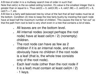
1. A B-tree of order m is a multiway search tree of order m such that: Note that ceil(x) is the so-called ceiling function. It's value is the smallest integer that is greater than or equal to x. Thus ceil(3) = 3, ceil(3.35) = 4, ceil(1.98) = 2, ceil(5.01) = 6, ceil(7) = 7, etc. A B-tree is a fairly well-balanced tree by virtue of the fact that all leaf nodes must be at the bottom. Condition (2) tries to keep the tree fairly bushy by insisting that each node have at least half the maximum number of children. This causes the tree to "fan out" so that the path from root to leaf is very short even in a tree that contains a lot of data.

2. Let's work our way through an example similar to that given by Kruse. Insert the following letters into what is originally an empty B-tree of order 5: C N G A H E K Q M F W L T Z D P R X Y S Order 5 means that a node can have a maximum of 5 children and 4 keys. All nodes other than the root must have a minimum of 2 keys. The first 4 letters get inserted into the same node, resulting in this picture:

3. When we try to insert the H, we find no room in this node, so we split it into 2 nodes, moving the median item G up into a new root node. Note that in practice we just leave the A and C in the current node and place the H and N into a new node to the right of the old one. Inserting E, K, and Q proceeds without requiring any splits:

4. Inserting M requires a split. Note that M happens to be the median key and so is moved up into the parent node. The letters F, W, L, and T are then added without needing any split.

5. When Z is added, the rightmost leaf must be split. The median item T is moved up into the parent node. Note that by moving up the median key, the tree is kept fairly balanced, with 2 keys in each of the resulting nodes. The insertion of D causes the leftmost leaf to be split. D happens to be the median key and so is the one moved up into the parent node. The letters P, R, X, and Y are then added without any need of splitting:

6. Finally, when S is added, the node with N, P, Q, and R splits, sending the median Q up to the parent. However, the parent node is full, so it splits, sending the median M up to form a new root node. Note how the 3 pointers from the old parent node stay in the revised node that contains D and G.

7. Deleting an Item In the B-tree as we left it at the end of the last section, delete H. Of course, we first do a lookup to find H. Since H is in a leaf and the leaf has more than the minimum number of keys, this is easy. We move the K over where the H had been and the L over where the K had been. This gives

8. Next, delete the T. Since T is not in a leaf, we find its successor (the next item in ascending order), which happens to be W, and move W up to replace the T. That way, what we really have to do is to delete W from the leaf, which we already know how to do, since this leaf has extra keys. In ALL cases we reduce deletion to a deletion in a leaf, by using this method Next, delete R. Although R is in a leaf, this leaf does not have an extra key; the deletion results in a node with only one key, which is not acceptable for a B-tree of order 5. If the sibling node to the immediate left or right has an extra key, we can then borrow a key from the parent and move a key up from this sibling. In our specific case, the sibling to the right has an extra key. So, the successor W of S (the last key in the node where the deletion occurred), is moved down from the parent, and the X is moved up. (Of course, the S is moved over so that the W can be inserted in its proper place.)

10. Finally, let's delete E. This one causes lots of problems. Although E is in a leaf, the leaf has no extra keys, nor do the siblings to the immediate right or left. In such a case the leaf has to be combined with one of these two siblings. This includes moving down the parent's key that was between those of these two leaves. In our example, let's combine the leaf containing F with the leaf containing A C. We also move down the D.

11. We begin by finding the immediate successor, which would be D, and move the D up to replace the C. However, this leaves us with a node with too few keys.

14. Topological Sort • Introduction. • Definition of Topological Sort. • Topological Sort is Not Unique. • Topological Sort Algorithm. • An Example. • Implementation. • Review Questions.

15. Introduction • There are many problems involving a set of tasks in which some of the tasks must be done before others. • For example, consider the problem of taking a course only after taking its prerequisites. • Is there any systematic way of linearly arranging the courses in the order that they should be taken? Yes! - Topological sort.

16. Definition of Topological Sort • Topological sort is a method of arranging the vertices in a directed acyclic graph (DAG), as a sequence, such that no vertex appear in the sequence before its predecessor. • The graph in (a) can be topologically sorted as in (b) (a) (b)

17. s1 = {a, b, c, d, e, f, g, h, i} s2 = {a, c, b, f, e, d, h, g, i} s3 = {a, b, d, c, e, g, f, h, i} s4 = {a, c, f, b, e, h, d, g, i} etc. Topological Sort is not unique • Topological sort is not unique. • The following are all topological sort of the graph below:

18. Topological Sort Algorithm • One way to find a topological sort is to consider in-degrees of the vertices. • The first vertex must have in-degree zero -- every DAG must have at least one vertex with in-degree zero. • The Topological sort algorithm is: • int topologicalOrderTraversal( ){ • int numVisitedVertices = 0; • while(there are more vertices to be visited){ • if(there is no vertex with in-degree 0) • break; • else{ • select a vertex v that has in-degree 0; • visit v; • numVisitedVertices++; • delete v and all its emanating edges; • } • } • return numVisitedVertices; • }

19. 1 3 2 0 2 A B C D E F G H I J 1 0 2 0 2 D G A B F H J E I C Topological Sort Example • Demonstrating Topological Sort.

20. Implementation of Topological Sort • The algorithm is implemented as a traversal method that visits the vertices in a topological sort order. • An array of length |V| is used to record the in-degrees of the vertices. Hence no need to remove vertices or edges. • A priority queue is used to keep track of vertices with in-degree zero that are not yet visited. public int topologicalOrderTraversal(Visitor visitor){ int numVerticesVisited = 0; int[] inDegree = new int[numberOfVertices]; for(int i = 0; i < numberOfVertices; i++) inDegree[i] = 0; Iterator p = getEdges(); while (p.hasNext()) { Edge edge = (Edge) p.next(); Vertex to = edge.getToVertex(); inDegree[getIndex(to)]++; }

21. Implementation of Topological Sort BinaryHeap queue = new BinaryHeap(numberOfVertices); p = getVertices(); while(p.hasNext()){ Vertex v = (Vertex)p.next(); if(inDegree[getIndex(v)] == 0) queue.enqueue(v); } while(!queue.isEmpty() && !visitor.isDone()){ Vertex v = (Vertex)queue.dequeueMin(); visitor.visit(v); numVerticesVisited++; p = v.getSuccessors(); while (p.hasNext()){ Vertex to = (Vertex) p.next(); if(--inDegree[getIndex(to)] == 0) queue.enqueue(to); } } return numVerticesVisited; }

22. Review Questions 1. List the order in which the nodes of the directed graph GB are visited by topological order traversal that starts from vertex a. 2. What kind of DAG has a unique topological sort? 3. Generate a directed graph using the required courses for your major. Now apply topological sort on the directed graph you obtained.

23. What is a Graph? • A graph G = (V,E) is composed of: V: set of vertices E: set ofedges connecting the vertices in V • An edge e = (u,v) is a pair of vertices • Example: a b V= {a,b,c,d,e} E= {(a,b),(a,c),(a,d), (b,e),(c,d),(c,e), (d,e)} c e d

24. JFK LAX LAX STL HNL DFW Applications CS16 • electronic circuits • networks (roads, flights, communications) FTL

25. Terminology: Adjacent and Incident • If (v0, v1) is an edge in an undirected graph, • v0 and v1 are adjacent • The edge (v0, v1) is incident on vertices v0 and v1 • If <v0, v1> is an edge in a directed graph • v0 is adjacent to v1, and v1 is adjacent from v0 • The edge <v0, v1> is incident on v0 and v1

26. Terminology:Degree of a Vertex • The degree of a vertex is the number of edges incident to that vertex • For directed graph, • the in-degree of a vertex v is the number of edgesthat have v as the head • the out-degree of a vertex v is the number of edgesthat have v as the tail • if di is the degree of a vertex i in a graph G with n vertices and e edges, the number of edges is Why? Since adjacent vertices each count the adjoining edge, it will be counted twice

27. Examples 0 3 2 1 2 0 3 3 1 2 3 3 6 5 4 3 1 G1 1 1 3 G2 1 3 0 in:1, out: 1 directed graph in-degree out-degree in: 1, out: 2 1 in: 1, out: 0 2 G3

28. Terminology:Path • path: sequence of vertices v1,v2,. . .vk such that consecutive vertices vi and vi+1 are adjacent. 3 2 3 3 3 a a b b c c e d e d a b e d c b e d c

29. More Terminology • simple path: no repeated vertices • cycle: simple path, except that the last vertex is the same as the first vertex a b b e c c e d

30. Even More Terminology • connected graph: any two vertices are connected by some path • subgraph: subset of vertices and edges forming a graph • connected component: maximal connected subgraph. E.g., the graph below has 3 connected components. connected not connected

31. Subgraphs Examples 0 1 2 0 0 3 1 2 1 2 3 0 0 0 0 1 1 1 2 2 0 1 2 3 G1 (i) (ii) (iii) (iv) (a) Some of the subgraph of G1 0 1 2 (i) (ii) (iii) (iv) (b) Some of the subgraph of G3 G3

32. More… • tree - connected graph without cycles • forest - collection of trees

33. Directed vs. Undirected Graph • An undirected graph is one in which the pair of vertices in a edge is unordered, (v0, v1) = (v1,v0) • A directed graph is one in which each edge is a directed pair of vertices, <v0, v1> != <v1,v0> tail head

34. Graph Representations • Adjacency Matrix • Adjacency Lists

35. Adjacency Matrix • Let G=(V,E) be a graph with n vertices. • The adjacency matrix of G is a two-dimensional n by n array, say adj_mat • If the edge (vi, vj) is in E(G), adj_mat[i][j]=1 • If there is no such edge in E(G), adj_mat[i][j]=0 • The adjacency matrix for an undirected graph is symmetric; the adjacency matrix for a digraph need not be symmetric

36. Examples for Adjacency Matrix 4 0 1 5 2 6 3 7 0 0 1 2 3 1 2 G2 G1 symmetric undirected: n2/2 directed: n2 G4

37. 0 0 4 1 2 5 6 3 7 1 2 3 0 1 2 3 1 1 2 3 2 0 1 2 3 4 5 6 7 0 2 3 0 3 0 1 3 0 3 1 2 1 2 0 5 G1 0 6 4 0 1 2 1 5 7 1 0 2 6 G4 G3 2 An undirected graph with n vertices and e edges ==> n head nodes and 2e list nodes

38. DFS is another popular search strategy. • It can do certain things that BFS cannot do. We will discuss some of these algorithms in COMP 271 (so you cannot get rid of DFS after COMP171). • DFS idea : • Whenever we visit a vertex v from another vertex u, we recursively visit a neighbor ofv that has not been visited before until all neighbors of v have been visited. Then we backtrack (return) to u. DFS : Depth-First Search Depth-First Search

39. Algorithm Flag all vertices as not visited Visit v, and mark v as visited. For each unvisited neighbor. make a recursive call RDFS(w). Depth-First Search

40. 0 8 2 9 1 7 3 6 4 5 Example Visited Table (T/F) Adjacency List source Pred Initialize visited table (all empty F) Initialize Pred to -1 Depth-First Search

41. 0 8 2 9 1 7 3 6 4 5 Example Visited Table (T/F) Adjacency List source Pred Mark 2 as visited visit sequence= {2} RDFS( 2 ) recursive call  RDFS(8) Depth-First Search

42. 0 8 2 9 1 7 3 6 4 5 Example Visited Table (T/F) Adjacency List source Pred visit sequence= {2, 8} Mark 8 as visited Recursivecalls RDFS( 2 ) RDFS(8) recursive callRDFS(0) Depth-First Search

43. 0 8 2 9 1 7 3 6 4 5 Example Visited Table (T/F) Adjacency List source Pred visit sequence= {2, 8, 0} Mark 0 as visited Recursivecalls RDFS( 2 ) RDFS(8) RDFS(0) -> no unvisited neighbor, return to (backtrack) RDFS(8) Depth-First Search

44. 0 8 2 9 1 7 3 6 4 5 Example Backtrack to 8 Visited Table (T/F) Adjacency List source Pred visit sequence= {2, 8, 0} Recursivecalls RDFS( 2 ) RDFS(8) recursive callRDFS(9) Depth-First Search

45. 0 8 2 9 1 7 3 6 4 5 Example Visited Table (T/F) Adjacency List source Pred visit sequence= {2, 8,0, 9} Mark 9 as visited Recursivecalls RDFS( 2 ) RDFS(8) RDFS(9) recursive callRDFS(1) Depth-First Search

46. 0 8 2 9 1 7 3 6 4 5 Example Visited Table (T/F) Adjacency List source Pred visit sequence= {2, 8,0,9, 1} Mark 1 as visited RDFS( 2 ) RDFS(8) RDFS(9) RDFS(1) recursive callRDFS(3) Recursivecalls Depth-First Search

47. 0 8 2 9 1 7 3 6 4 5 Example Visited Table (T/F) Adjacency List source RDFS( 2 ) RDFS(8) RDFS(9) RDFS(1) RDFS(3) recursive callRDFS(4) Pred visit sequence= {2, 8,0,9, 1, 3} Mark 3 as visited Recursivecalls Depth-First Search

48. 0 8 2 9 1 7 3 6 4 5 Example Visited Table (T/F) Adjacency List source RDFS( 2 ) RDFS(8) RDFS(9) RDFS(1) RDFS(3) RDFS(4)  STOP all of 4’s neighbors have been visited backtrack (return back) to call RDFS(3) visit sequence= {2, 8,0,9, 1,3, 4} Pred Mark 4 as visited Recursivecalls Depth-First Search

49. 0 8 2 9 1 7 3 6 4 5 Example Visited Table (T/F) Adjacency List source Backtrack to 3 visit sequence= {2, 8,0,9, 1,3,4} Pred RDFS( 2 ) RDFS(8) RDFS(9) RDFS(1) RDFS(3) recursive callRDFS(5) Recursivecalls Depth-First Search

50. 0 8 2 9 1 7 3 6 4 5 Example Visited Table (T/F) Adjacency List source RDFS( 2 ) RDFS(8) RDFS(9) RDFS(1) RDFS(3) RDFS(5) 3 is visited, recursive callRDFS(6) visit sequence= {2, 8,0,9, 1,3,4, 5} Pred Mark 5 as visited Recursivecalls Depth-First Search