Download
1 / 50
510 likes | 727 Vues
Chapter 1: The Big Picture. The Layers of a Computing System. Chapter 1 The Big Picture Page 1. History of Computer Science. The Abacus

E N D
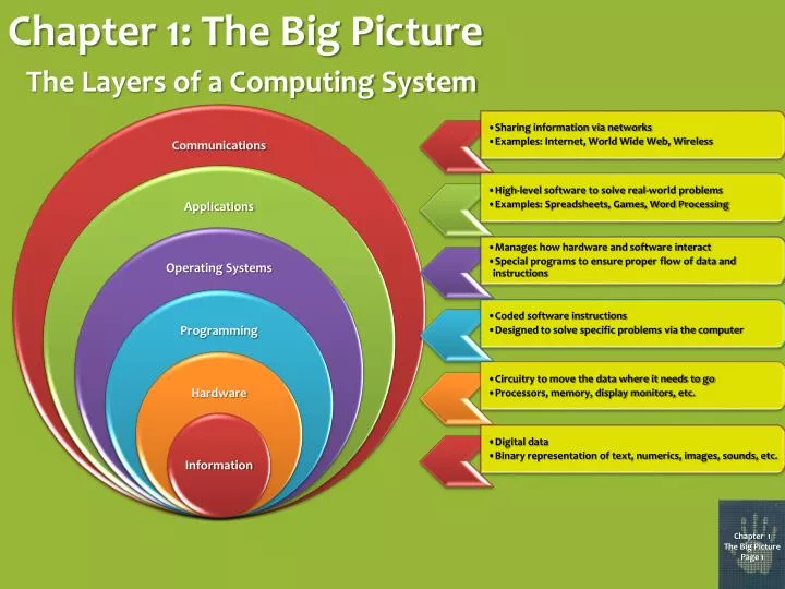
Chapter 1: The Big Picture The Layers of a Computing System Chapter 1 The Big Picture Page 1
History of Computer Science The Abacus Originally developed by the Babylonians around 2400 BC, this arithmetic calculating tool was also used by ancient Egyptians, Greeks, Romans, Indians, and Chinese. The Algorithm In the year 825, the Persian mathematician Muhammad ibnMūsā al-Khwārizmī developed the concept of performing a series of steps in order to accomplish a task, such as the systematic application of arithmetic to algebra. Chapter 1 The Big Picture Page 2
History of Computer Science The Analytical Engine Designed by British mathematician Charles Babbage in the mid-19th century, this steam-powered mechanical device (never successfully built) had the functionality of today’s modern computers. Binary Logic Also in the mid-1800’s, British mathematician George Boole developed a complete algebraic system that allowed computational processes to be mathematically modeled with zeros and ones (representing true/false, on/off, etc.). Chapter 1 The Big Picture Page 3
History of Computer Science Computability In the early 20th century, American mathematician Alonzo Church and British mathematician Alan Turing independently developed the thesis that a mathematical method is effective if it could be set out as a list of instructions able to be followed by a human clerk (a “computer”) with paper and pencil, for as long as necessary, and without ingenuity or insight. Turing Machine In 1936, Turing developed a mathematical model for an extremely basic abstract symbol-manipulating device which, despite its simplicity, could be adapted to simulate the logic of any computer that could possibly be constructed. Chapter 1 The Big Picture Page 4
History of Computer Science Digital Circuit Design In 1937, Claude Shannon, an American electrical engineer, recognized that Boolean algebra could be used to arrange electromechanical relays, which were then used in telephone routing switches, to solve logic problems, the basic concept underlying all electronic digital computers. Cybernetics During World War II, American mathematician Norbert Wiener experimented with anti-aircraft systems that automatically interpreted radar images to detect enemy planes. This approach of developing artificial systems by examining real systems became known as cybernetics. Chapter 1 The Big Picture Page 5
History of Computer Science Transistor The fundamental building block of the circuitry in modern electronic devices was developed in the early 1950s. Because of its fast response and accuracy, the transistor is used in a wide variety of digital and analog functions, including switching, amplification, voltage regulation, and signal modulation. Programming Languages In 1957, IBM released the Fortran programming language (the IBM Mathematical Formula Translating System), designed to facilitate numerical computation and scientific computing. In 1958, a committee of European and American scientists developed ALGOL, the Algorithmic Language, which pioneered the language design features that characterize most modern languages. In 1959, under the supervision of the U.S. Department of Defense, a consortium of technology companies (IBM, RCA, Sylvania, Honeywell, Burroughs, and Sperry-Rand) developed COBOL, the Common Business-Oriented Language, to help develop business, financial, and administrative systems for companies and governments. Chapter 1 The Big Picture Page 6
History of Computer Science Operating Systems In 1964, IBM’s System 360 mainframe computers utilized a single operating system (rather than using separate ad hoc systems for each machine) to schedule and manage the execution of different jobs on the computer. Mouse In 1967, Stanford’s Douglas Engelbart employed a wooden case and two metal wheels to invent his “X-Y Position Indicator for a Display System”. Chapter 1 The Big Picture Page 7
History of Computer Science Relational Databases In 1969, IBM’s Edgar Codd developed a table-based model for organizing data in large systems so it could be easily accessed. Computational Complexity In 1971, American computer scientist Stephen Cook pioneered research into NP-completeness, the notion that some problems may not be solvable on a computer in a “reasonable” amount of time. Supercomputers In 1976, Seymour Cray developed the first computer to utilize multiple processors in order to vastly accelerate the computation of extremely complex scientific calculations. Personal Computers In 1976, Steve Jobs and Steve Wozniak formed Apple Computer, Inc., facilitating the capability of purchasing a computer for home use. Chapter 1 The Big Picture Page 8
History of Computer Science Internet In 1969, DARPA (the Defense Advanced Research Projects Agency) established ARPANET as a computer communication network that did not require dedicated lines between every pair of communicating terminals. By 1977, ARPANET had grown from its initial four nodes in California and Utah to over 100 nodes nationwide. In 1988, the National Science Foundation established five supercomputer centers and connected them via ARPANET in order to provide supercomputer access to academic researchers nationwide. By 1995, private sector entities had begun to find it profitable to build and expand the Internet’s infrastructure, so NSFNET was retired and the Internet backbone was officially privatized. Chapter 1 The Big Picture Page 9
History of Computer Science • Microsoft • In 1975, Bill Gates and Paul Allen founded the software company that would ultimately achieve numerous milestones in the history of computer science: • 1981: Contracted with IBM to produce DOS (Disk Operating System) for use in IBM’s new line of personal computers. • 1985: Introduced Microsoft Windows, providing PC users with a graphical user interface, which promoted ease of use in PCs. (Resulted in “look-and-feel” lawsuit from Apple.) • 1989: Released Microsoft Office, a suite of office productivity applications, including Microsoft Word and Microsoft Excel. (Accused of unfairly exploiting its knowledge of underlying operating systems by office suite competitors.) • 1995: Entered Web browser market with Internet Explorer. (Criticized for security flaws and lack of compliance with many Web standards.) Chapter 1 The Big Picture Page 10
Chapter 2: Binary Values and Number Systems • Information may be reduced to its fundamental state by means of binary numbers (e.g., on/off, true/false, yes/no, high/low, positive/negative). • “Bits” (binary digits) are used to accomplish this. Normally, we consider a binary value of 1 to represent a “high” state, while a binary value of 0 represents a “low” state. • In machines, these values are represented electronically by high and low voltages, and magnetically by positive and negative polarities. 0 1 0 1 0 0 1 1 0 1 0 1 0 Chapter 2 Binary Values and Number Systems Page 11
Binary Numerical Expressions • Binary expressions with multiple digits may be viewed in the same way that multi-digit decimal numbers are viewed, except in base 2 instead of base 10. • For example, just as the decimal number 275 is viewed as 5 ones, 7 tens, and 2 hundreds combined, the binary number 01010110 can be viewed in right-to-left fashion as... 01010110 01010110 01010110 01010110 01010110 01010110 01010110 01010110 01010110 01010110 • 0 ones So, 01010110 is equivalent to the decimal number 2 + 4 + 16 + 64 = 86 • 1 two • 1 four • 0 eights • 1 sixteen • 0 thirty-twos • 1 sixty-four • 0 one hundred twenty-eights Chapter 2 Binary Values and Number Systems Page 12
Hexadecimal (Base-16) Notation • As a shorthand way of writing lengthy binary codes, computer scientists often use hexadecimal notation. For example, the binary expression 1011001011101000 may be written in hexadecimal notation as B2E8. The two expressions mean the same thing, but they are in different notations. Chapter 2 Binary Values and Number Systems Page 13
Chapter 3: Data Representation Computers use bits to represent all types of data, including text, numerical values, sounds, images, and animation. How many bits does it take to represent a piece of data that could have one of, say, 1000 values? • If only one bit is used, then there are only two possible values: 0 and 1. • If two bits are used, then there are four possible values: 00, 01, 10, and 11. • Three bits produces eight possible values: 000, 001, 010, 011, 100, 101, 110 and 111. • Four bits produces 16 values; five bits produces 32; six produces 64; ... • Continuing in this fashion, we see that k bits would produce 2k possible values. • Since 29 is 512 and 210 is 1024, we would need ten bits to represent a piece of data that could have one of 1000 values. • Mathematically, this is the “ceiling” of the base-two logarithm, i.e., the count of how many times you could divide by two until you get to the value one: Chapter 3 Data Representation Page 14
Representing Integers with Bits Two’s complement notation was established to ensure that addition between positive and negative integers shall follow the logical pattern. 1 1 1 1 1 1 1 1 1 1 1 1 0 0 1 0 1 1 0 1 1 1 0 0 0 0 1 1 0 1 Examples: + + + + + 0 1 0 1 0 0 0 1 1 0 1 0 1 1 1 0 1 1 0 1 1 1 0 0 0 1 0 0 0 1 0 0 0 1 0 1 1 1 1 0 -3 + 3 = 0 3 + 2 = 5 -4 + -3 = -7 6 + 3 = -7??? OVERFLOW! -7 + -2 = 7??? OVERFLOW! Chapter 3 Data Representation Page 15
Two’s Complement Coding & Decoding • How do we code –44 in two’s complement notation using 8 bits? • First, write the value 44 in binary using 8 bits:00101100 • Starting on the right side, skip over all zeros and the first one:00101100 • Continue moving left, complementing each bit:11010100 • The result is -44 in 8-bit two’s complement notation: 11010100 • How do we decode 10110100 from two’s complement into an integer? • Starting on the right side, skip over all zeros and the first one: 10110100 • Continue moving left, complementing each bit: 01001100 • Finally, convert the resulting positive bit code into an integer: 76 • So, the original negative bit code must have represented: –76 Chapter 3 Data Representation Page 16
Representing Real Numbers with Bits • When representing a real number like 17.15 in binary form, a rather complicated approach is taken. • Using only powers of two, we note that 17 is 24 + 20 and .15 is 2-3 + 2-6 + 2-7 + 2-10 + 2-11 + 2-14 + 2-15 + 2-18 + 2-19 + 2-22 + … • So, in pure binary form, 17.15 would be 10001.0010011001100110011001… • In “scientific notation”, this would be 1.0001001001100110011001… × 24 • The standard for floating-point notation is to use 32 bits. The first bit is a sign bit(0 for positive, 1 for negative). The next eight are a bias-127 exponent (i.e., 127 + the actual exponent). And the last 23 bits are the mantissa (i.e., the exponent-less scientific notation value, without the leading 1). • So, 17.15 would have the following floating-point notation: 0 10000011 00010010011001100110011 Chapter 3 Data Representation Page 17
Representing Text with Bits ASCII: American Standard Code for Information Interchange 0000000 NUL (null) 0100000 SPACE 1000000 @ 1100000 ` 0000001 SOH (start of heading) 0100001 ! 1000001 A 1100001 a 0000010 STX (start of text) 0100010 " 1000010 B 1100010 b 0000011 ETX (end of text) 0100011 # 1000011 C 1100011 c 0000100 EOT (end of transmission) 0100100 $ 1000100 D 1100100 d 0000101 ENQ (enquiry) 0100101 % 1000101 E 1100101 e 0000110 ACK (acknowledge) 0100110 & 1000110 F 1100110 f 0000111 BEL (bell) 0100111 ' 1000111 G 1100111 g 0001000 BS (backspace) 0101000 ( 1001000 H 1101000 h 0001001 TAB (horizontal tab) 0101001 ) 1001001 I 1101001 i 0001010 LF (NL line feed, new line) 0101010 * 1001010 J 1101010 j 0001011 VT (vertical tab) 0101011 + 1001011 K 1101011 k 0001100 FF (NP form feed, new page) 0101100 , 1001100 L 1101100 l 0001101 CR (carriage return) 0101101 - 1001101 M 1101101 m 0001110 SO (shift out) 0101110 . 1001110 N 1101110 n 0001111 SI (shift in) 0101111 / 1001111 O 1101111 o 0010000 DLE (data link escape) 0110000 0 1010000 P 1110000 p 0010001 DC1 (device control 1) 0110001 1 1010001 Q 1110001 q 0010010 DC2 (device control 2) 0110010 2 1010010 R 1110010 r 0010011 DC3 (device control 3) 0110011 3 1010011 S 1110011 s 0010100 DC4 (device control 4) 0110100 4 1010100 T 1110100 t 0010101 NAK (negative acknowledge) 0110101 5 1010101 U 1110101 u 0010110 SYN (synchronous idle) 0110110 6 1010110 V 1110110 v 0010111 ETB (end of trans. block) 0110111 7 1010111 W 1110111 w 0011000 CAN (cancel) 0111000 8 1011000 X 1111000 x 0011001 EM (end of medium) 0111001 9 1011001 Y 1111001 y 0011010 SUB (substitute) 0111010 : 1011010 Z 1111010 z 0011011 ESC (escape) 0111011 ; 1011011 [ 1111011 { 0011100 FS (file separator) 0111100 < 1011100 \ 1111100 | 0011101 GS (group separator) 0111101 = 1011101 ] 1111101 } 0011110 RS (record separator) 0111110 > 1011110 ^ 1111110 ~ 0011111 US (unit separator) 0111111 ? 1011111 _ 1111111 DEL • ASCII code was developed as a means of converting text into a binary notation. • Each character has a 7-bit representation. • For example, CAT would be represented by the bits: 100001110000011010100 Chapter 3 Data Representation Page 18
Fax Machines In order to transmit a facsimile of a document over telephone lines, fax machines were developed to essentially convert the document into a grid of tiny black and white rectangles. This important document must be faxed immediately!!! A standard 8.511 page is divided into 1145 rows and 1728 columns, producing approximately 2 million 0.0050.01 rectangles. Each rectangle is scanned by the transmitting fax machine and determined to be either predominantly white or predominantly black. We could just use the binary nature of this black/white approach (e.g., 1 for black, 0 for white) to fax the document, but that would require 2 million bits per page! Chapter 3 Data Representation Page 19
CCITT Fax Conversion Code By using one sequence of bits to represent a long run of a single color (either black or white), the fax code can be compressed to a fraction of the two million bit code that would otherwise be needed. length whiteblack 0 001101010000110111 1 000111010 2 011111 3 100010 4 1011011 5 11000011 6 11100010 7 111100011 8 10011000101 9 10100000100 10 001110000100 11 010000000101 12 0010000000111 13 00001100000100 14 11010000000111 15 110101000011000 16 1010100000010111 17 1010110000011000 18 01001110000001000 19 00011000000100111 20 000100000001101000 21 001011100001101100 22 000001100000110111 23 000001100000101000 24 010100000000010111 25 010101100000011000 26 0010011000011001010 27 0100100000011001011 28 0011000000011001100 29 00000010000011001101 30 00000011000001101000 31 00011010000001101001 32 00011011000001101010 33 00010010000001101011 34 00010011000011010010 length whiteblack 35 00010100000011010011 36 00010101000011010100 37 00010110000011010101 38 00010111000011010110 39 00101000000011010111 40 00101001000001101100 41 00101010000001101101 42 00101011000011011010 43 00101100000011011011 44 00101101000001010100 45 00000100000001010101 46 00000101000001010110 47 00001010000001010111 48 00001011000001100100 49 01010010000001100101 50 01010011000001010010 51 01010100000001010011 52 01010101000000100100 53 00100100000000110111 54 00100101000000111000 55 01011000000000100111 56 01011001000000101000 57 01011010000001011000 58 01011011000001011001 59 01001010000000101011 60 01001011000000101100 61 00110010000001011010 62 00110011000001100110 63 00110100000001100111 64 11011000000111 128 10010000011001000 192 010111000011001001 256 0110111000001011011 320 00110110000000110011 384 00110111000000110100 length whiteblack 448 01100100000000110101 512 011001010000001101100 576 01101000 0000001101101 640 01100111 0000001001010 704 0110011000000001001011 768 0110011010000001001100 832 0110100100000001001101 896 0110100110000001110010 960 0110101000000001110011 1024 0110101010000001110100 1088 0110101100000001110101 1152 011010111 0000001110110 1216 0110110000000001110111 1280 011011001 0000001010010 1344 0110110100000001010011 1408 011011011 0000001010100 1472 010011000 0000001010101 1536 010011001 0000001011010 1600 010011010 0000001011011 1664 0110000000001100100 1728 010011011 0000001100101 1792 00000001000 00000001000 1856 0000000110000000001100 1920 00000001101 00000001101 1984 000000010010000000010010 2048 000000010011000000010011 2112 000000010100000000010100 2176 000000010101000000010101 2240 000000010110000000010110 2304 000000010111000000010111 2368 000000011100000000011100 2432 000000011101000000011101 2496 000000011110000000011110 2560 000000011111000000011111 Chapter 3 Data Representation Page 20
Binary Code Interpretation How is the following binary code interpreted? 10100111101111010000011001011100001111001111110010101110 In “programmer’s shorthand” (hexadecimal notation)… 1111 1100 1010 0111 1011 1101 0000 0110 0101 1100 0011 1100 1010 1110 F C A 7 B D 0 6 5 C 3 C A E As a two’s complement integer... The negation of 01011000010000101111100110100011110000110000001101010010 (21+24+26+28+29+216+217+222+223+224+225+229+231+232+235+236+237+238+239+241+246+251+252+254) -24,843,437,912,294,226 As ASCII text… 1010011 1101111 0100000 1100101 1100001 1110011 1111001 0101100 S o (space) e a s y . As CCITT fax conversion code… 10 3 black 10 3 black 11 2 black 00011 7 black 0000111 12 black 11 2 black 10100 9 white 11011 64 white 110100 14 white 0010111 21 white 10011 6 white 1100 5 white 1011 4 white Chapter 3 Data Representation Page 21
Representing Audio Data with Bits Audio files are digitized by sampling the audio signal thousands of times per second and then “quantizing” each sample (i.e., rounding off to one of several discrete values). The ability to recreate the original analog audio depends on the resolution (i.e., the number of quantization levels used) and the sampling rate. Chapter 3 Data Representation Page 22
Representing Still Images with Bits Digital images are composed of three fields of color intensity measurements, separated into a grid of thousands of pixels (picture elements) . The size of the grid (the image’s resolution) determines how clear the image can be displayed. 2 2 4 4 8 8 16 16 32 32 64 64 128 128 256 256 512 512 Chapter 3 Data Representation Page 23
RGB Color Representation In digital display systems, each pixel in an image is represented as an additive combination of the three primary color components: red, green, and blue. Printers, however, use a subtractive color system, in which the complementary colors of red, green, and blue (cyan, magenta, and yellow) are applied in inks and toners in order to subtract colors from a viewer’s perception. Chapter 3 Data Representation Page 24
Compressing Images with JPEG The Joint Photographic Experts Group developed an elaborate procedure for compressing color image files: Each square is split into three 88 grids indicating the levels of lighting and blue and red coloration the square contains. First, the original image is split into 88 squares of pixels. Depending on how severely the values were rounded, the restored image will either be a good representation of the original (with a high bit count) or a bad representation (with a low bit count). After rounding off the values in the three grids in order to reduce the number of bits needed, each grid is traversed in a zig-zag pattern to maximize the chances that consecutive values will be equal, which, as occurred in fax machines, reduces the bit requirement even further. Chapter 3 Data Representation Page 25
Representing Video with Bits Video images are merely a sequence of still images, shown in rapid succession. One means of compressing such a vast amount of data is to use the JPEG technique on each frame, thus exploiting each image’s spatial redundancy. The resulting image frames are called intra-frames. Video also possesses temporal redundancy, i.e., consecutive frames are usually nearly identical, with only a small percentage of the pixels changing color significantly. So video can be compressed further by periodically replacing several I-frames with predictive frames, which only contain the differences between the predictive frame and the last I-frame in the sequence. P-frames are generally about one-third the size of corresponding I-frames. The Motion Picture Experts Group (MPEG) went even further by using bidirectional frames sandwiched between I-frames and P-frames (and between consecutive P-frames). Each B-frame includes just enough information to allow the original frame to be recreated by blending the previous and next I/P-frames. B-frames are generally about half as big as the corresponding P-frames (i.e., one-sixth the size of the corresponding I-frames). Chapter 3 Data Representation Page 26
Chapter 4: Gates and Circuits The following Boolean operations are easy to incorporate into circuitry and can form the building blocks of many more sophisticated operations… The NOT Operation (i.e., what’s the opposite of the operand’s value?) NOT 1 = 0 NOT 0 = 1 NOT 10101001 = 01010110 NOT 00001111 = 11110000 The AND Operation (i.e., are both operands “true”?) 1 AND 1 1 1 AND 0 0 0 AND 1 0 0 AND 0 0 10101001 AND 10011100 10001000 00001111 AND 10110101 00000101 The OR Operation (i.e., is either operand “true”?) 1 OR 1 1 1 OR 0 1 0 OR 1 1 0 OR 0 0 10101001 OR 10011100 10111101 00001111 OR 10110101 10111111 Chapter 4 Gates and Circuits Page 27
More Boolean Operators The NAND Operation (“NOT AND”) 1 NAND 1 0 1 NAND 0 1 0 NAND 1 1 0 NAND 0 1 10101001 NAND 10011100 01110111 00001111 NAND 10110101 11111010 The NOR Operation (“NOT OR”) 1 NOR 1 0 1 NOR 0 0 0 NOR 1 0 0 NOR 0 1 10101001 NOR 10011100 01000010 00001111 NOR 10110101 01000000 The XOR Operation (“Exclusive OR”, i.e, either but not both is “true”) 1 XOR 1 0 1 XOR 0 1 0 XOR 1 1 0 XOR 0 0 10101001 XOR 10011100 00110101 00001111 XOR 10110101 10111010 Chapter 4 Gates and Circuits Page 28
Transistors Transistors are relatively inexpensive mechanisms for implementing the Boolean operators. In addition to the input connection (the base), transistors are connected to both a power source and a voltage dissipating ground. Essentially, when the input voltage is high, an electric path is formed within the transistor that causes the power source to be drained to ground. When the input voltage is low, the path is not created, so the power source is not drained. Chapter 4 Gates and Circuits Page 29
Using Transistors to Create Logic Gates A NOT gate is essentially implemented by a transistor all by itself. A NAND gate uses a slightly more complex setup in which both inputs would have to be high to force the power source to be grounded. Use the output of a NAND gate as the input to a NOT gate to produce an AND gate. A NOR gate grounds the power source if either or both of the inputs are high. Use the output of a NOR gate as the input to a NOT gate to produce an OR gate. Chapter 4 Gates and Circuits Page 30
How to Use Logic Gates for Arithmetic ANDs and ORs are all well and good, but how can they be used to produce binary arithmetic? Let’s start with simple one-bit addition (with a “carry” bit just in case someone tries to add 1 + 1!). Notice that the sum bit always yields the same result as the XOR operation, and the carry bit always yields the same result as the AND operation! By combining the right circuitry, then, multiple-bit addition can be implemented, as well as the other arithmetic operations. Chapter 4 Gates and Circuits Page 31
Memory Circuitry With voltages constantly on the move, how can a piece of circuitry be used to retain a piece of information? In the S-R latch, as long as the S and R inputs remain at one, the value of the Q output will never change, i.e., the circuit serves as memory! To set the stored value to one, merely set the S input to zero (for just an instant!) while leaving the R input at one. To set the stored value to zero, merely set the R input to zero (for just an instant!) while leaving the S input at one. Question: What goes wrong if both inputs are set to zero simultaneously? Chapter 4 Gates and Circuits Page 32
Chapter 5: Computing Components In the 1940s and 1950s, John von Neumann helped develop the architecture that continues to be used in the design of most modern computer systems. Control Unit, Coordinating CPU Activity Arithmetic/ Logic Unit, Processing Data Chapter 5 Computing Components Page 33
Central Processing Unit (CPU) Code Cache Storage for instructions for deciphering data Branch Predictor Unit Decides which ALU can best handle specific data & divides the tasks Bus Interface Unit Information from the RAM enters the CPU here , and then it is sent to separate storage units or cache Instruction Prefetch & Decoding Unit Translates data into simple instructions for ALU to process Arithmetic Logic Unit Whole number cruncher Floating Point Unit Floating-point number cruncher Data Cache Sends data from ALUs to Bus Interface Unit, and then back to RAM Instruction Register Provides the ALUs with processing instructions from the data cache Chapter 5 Computing Components Page 34
Simplified View of the CPU CPU RAM Registers Special memory cells to temporarily store the data being manipulated Control Unit Circuitry to coordinate the operation of the computer ALU Circuitry that manipulates the data Bus Chapter 5 Computing Components Page 35
The Processing Cycle DECODE instruction to determine what to do CONTROL UNIT ARITHMETIC/LOGIC UNIT EXECUTE the decoded instruction FETCH the next instruction from main memory STORE the result in main memory MAIN MEMORY Chapter 5 Computing Components Page 36
Sample Machine Architecture Main Memory Cells : : Registers Control Unit 00 EE 01 EF 02 F0 0 03 F1 1 Program Counter (Keeps track of the address of the next instruction to be executed) 04 F2 2 05 F3 3 06 F4 4 07 F5 5 08 F6 6 09 F7 7 0A F8 8 0B F9 9 0C Instruction Register (Contains a copy of the 2-byte instruction currently being executed) FA A 0D FB B 0E FC C 0F FD D 10 FE E 11 FF F : : CPU ALU Bus Chapter 5 Computing Components Page 37
Random Access Memory (RAM) • Whenever a computer accesses information (e.g., a program that’s being executed, data that’s being examined), that information is stored as electronic pulses within main memory. • Main memory is a system of electronic circuits known as random access memory (RAM), the idea being that the user can randomly access any part of memory (as long as the location of what’s being accessed is known). • The circuitry in main memory is usually dynamic RAM, meaning that the binary values must be continuously refreshed (thousands of times per second) or the charge will dissipate and the values will be lost. Chapter 5 Computing Components Page 38
Cache Memory • Due to the need for continuous refreshing, dynamic RAM is rather slow. An alternative approach is static RAM, which uses “flip-flop” circuitry that doesn’t waste time refreshing the stored binary values. • Static RAM is much faster than dynamic RAM, but is much more expensive. Consequently, it is used less in most machines. • Cache memory uses static RAM as the first place to look for information and as the place to store the information that was most recently accessed (e.g., the current program being executed). Chapter 5 Computing Components Page 39
Magnetic Memory • When the power is turned off, a computer’s electronic memory devices immediately lose their data. In order to store information on a computer when it’s turned off, some non-magnetic storage capability is required. • Most computers contain hard drives, a system of magnetic platters and read-write heads that detect the polarity of the magnetic filaments beneath them (i.e., “reading” the bit values) and induce a magnetic field onto the filaments (i.e., “writing” the bit values). Chapter 5 Computing Components Page 40
Disk Tracks and Sectors • Each platter is divided into concentric circles, called tracks, and each track is divided into wedges, called sectors. • The read-write head moves radially towards and away from the center of the platter until it reaches the right track. • The disk spins around until the read-write head reaches the appropriate sector. Chapter 5 Computing Components Page 41
Optical Memory • Compact Disks – Read-Only Memory (CD-ROMs) use pitted disks and lasers to store binary information. • When the laser hits an unpitted “land”, light is reflected to a sensor and interpreted as a 1-bit; when the laser hits a pit, light isn’t reflected back, so it’s interpreted as a 0-bit. • Digital Versatile Disks (DVDs) use the same pits-and-lands approach as CD-ROMs, but with finer gaps between tracks and pits, resulting in over four times the storage capacity as CD-ROMs. Chapter 5 Computing Components Page 42
Flash Memory • Recent advances in memory circuitry have made it possible to develop portable electronic devices with large memory capacities. • Flash memory is Electrically Erasable Programmable Read-Only Memory (EEPROM): • Read-Only Memory: Non-volatile (retains data even after power is shut off), but difficult to alter. • Programmable: Programs aren’t added until after the device is manufactured, by “blowing” all fuses for which a 1-value is desired. • Electrically Erasable: Erasing is possible by applying high electric fields. USB Mass Storage Controller Flash Memory Chip Universal Serial Bus (USB) Connector to Host Computer Test Points for Verifying Proper Loading LEDs to Indicate Data Transfers Crystal Oscillator to Produce Clock Signal Space for Second Flash Memory Chip Write-Protect Switch Chapter 5 Computing Components Page 43
Input Device: Keyboard One of the principal devices for providing input to a computer is the keyboard. When a key is pressed, a plunger on the bottom of the key pushes down against a rubber dome… …the center of which completes a circuit within the keyboard, resulting in the CPU being signaled regarding which key (or keys) has been pressed. Chapter 5 Computing Components Page 44
Input Device: Mouse The other primary input device is the computer mouse. Optical Mouse Mechanical Mouse Moving the mouse turns the ball The mouse driver software processes the X and Y data and transfers it to the operating system X and Y rollers grip the ball and transfer movement Optical encoding disks include light holes Optical mice use red LEDs (or lasers) to illuminate the surface beneath the mouse, and sensors detect the subtle changes that indicate how much and in what direction the mouse is being moved. Sensors gather light pulses to convert to X and Y velocities Infrared LEDs shine through the disks Chapter 5 Computing Components Page 45
Output Device: Cathode Ray Tube (CRT) Deflection Coils These magnetic plates deflect the beams horizontally and vertically to particular screen coordinates Anode Connection The positive charge on the anode attracts the electrons and accelerates them forwards Focusing Coil The magnetic coil forces the electron flows to focus into tight beams Electron Guns A heating filament releases electrons from a cathode, which flow through a control grid (controlling brightness) Shadow Mask A perforated metal sheet halts stray electrons and ensures that beams focus upon target phosphors Phosphor-Coated Screen Each pixel is comprised of a triad of RGB phosphors that are illuminated by the three electron beams Chapter 5 Computing Components Page 46
Output Device: Liquid Crystal Display Color Filter Provides red, green, or blue color to resulting light Twisted Nematic Liquid Crystals Twists shaft of light 90º when uncharged, 0º when fully charged Light Source Vertical Polarizer Amount of light permitted to pass is proportional to how close to vertical its shafts are Thin Film Transistor Applies charge to individual subpixel Horizontal Polarizer Converts light into horizontal shafts Chapter 5 Computing Components Page 47
Output Device: Plasma Display Dielectric Layer Contains transparent display electrodes, arranged in long vertical columns Plasma Cells Phosphor coating is excited by plasma ionization and photon release Pixel Comprised of three plasma cells, one of each RGB phosphor coating Rear Plate Glass Dielectric Layer Contains transparent address electrodes, arranged in long horizontal rows Front Plate Glass Chapter 5 Computing Components Page 48
Input/Output Device: Touch Screen Resistive The glass layer has an outer coating of conductive material, and insulating dots separate it from a flexible membrane with an inner conductive coating. When the screen is touched, the two conductive materials meet, producing a locatable voltage. Capacitive Small amounts of voltage are applied to the four corners of the screen. Touching the screen draws current from each corner, and a controller measures the ratio of the four currents to determine the touch location. Infrared A small frame is placed around the display, with infrared LEDs and photoreceptors on opposite sides. Touching the screen breaks beams that identify the specific X and Y coordinates. Acoustic Four ultrasonic devices are placed around the display. When the screen is touched, an acoustic pattern is produced and compared to the patterns corresponding to each screen position. Chapter 5 Computing Components Page 49
Parallel Processing Traditional computers have a single processor. They execute one instruction at a time and can deal with only one piece of data at a time. These machines are said to have SISD (Single Instruction, Single Data) architectures. When multiple processors are applied within a single computer, parallel processing can take place. There are two basic approaches used in these “supercomputers”: • MIMD (Multiple Instruction, Multiple Data) Architectures • At any given moment, each processor does its own task to its own portion of the data • Example: Have some processors retrieve data, some perform calculations, and some render the resulting images: • SIMD (Single Instruction, Multiple Data) Architectures • Each processor does the same thing at the same time to its own portion of the data • Example: Have the processors perform the graphics rendering for different sectors of the viewscreen: Chapter 5 Computing Components Page 50