Download
1 / 74
740 likes | 836 Vues
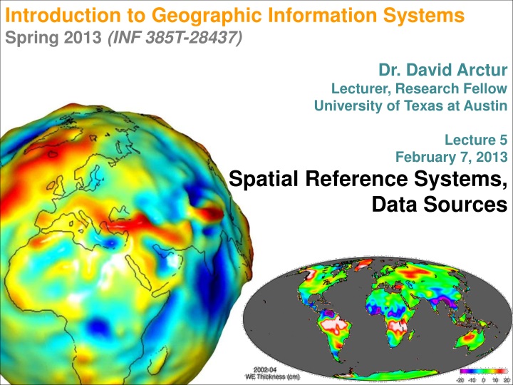
Introduction to Geographic Information Systems Spring 2013 (INF 385T-28437) Dr. David Arctur Lecturer, Research Fellow University of Texas at Austin Lecture 5 February 7, 2013 Spatial Reference Systems, Data S ources. Outline. Models of the Earth Map projections Coordinate systems

E N D
Introduction to Geographic Information Systems Spring 2013 (INF 385T-28437) Dr. David Arctur Lecturer, Research Fellow University of Texas at Austin Lecture 5 February 7, 2013 Spatial Reference Systems, Data Sources
Outline • Models of the Earth • Map projections • Coordinate systems • GIS data sources • Vector data formats • Raster data formats INF385T(28437) – Spring 2013 – Lecture 5
Models of the Earth’s shape INF385T(28437) – Spring 2013 – Lecture 5 • Sphere with radius of ~6378 km • Ellipsoid (or Spheroid) with equatorial radius (semimajor axis) of ~6378 km and polar radius (semiminor axis) of ~6357 km • Difference of ~21km usually expressed as “flattening” (f) ratio of the ellipsoid: • f= difference / major axis = ~ 1/300 for Earth • and “inverse flattening” would be ~300
Ellipsoid dimensions and flattening Ellipsoid = Spheroid in GIS… INF385T(28437) – Spring 2013 – Lecture 5
Ellipsoid vs Geoid vs Datum • The Geoidis approximately where sea level would be throughout the world (measured by plumb bob away from coastal areas) • Due to variations in the Earth’s gravity field, this “global sea level” would not fit any one ellipsoid, as evident in figure • Datum= shape of ellipsoid AND location of origin for axis of rotation relative to Earth center of mass
Horizontal Control Datums INF385T(28437) – Spring 2013 – Lecture 5 Commons North American Datums • NAD27(1927 North American Datum) • Clarke (1866) ellipsoid, non-geocentric (local origin) for axis of rotation • NAD83(1983 North American Datum) • GRS80 ellipsoid, geocentric origin for axis of rotation • WGS84(1984 World Geodetic System) • WGS84 ellipsoid, geocentric, nearly identical to NAD83 • Other datums are also in use globally
Datum shifts INF385T(28437) – Spring 2013 – Lecture 5
Datum transformations INF385T(28437) – Spring 2013 – Lecture 5 Theoretical method: use equations relating Lat/Lon in one datum to another Empirical method: use grid of differences to convert values directly from one datum to another See Esri digital book on Map Projections for more information
How do we get from 3D Earth to 2D maps??? Map projections INF385T(28437) – Spring 2013 – Lecture 5
Latitude and longitude INF385T(28437) – Spring 2013 – Lecture 5 Longitude (meridians)
Latitude and longitude INF385T(28437) – Spring 2013 – Lecture 5 Latitude (parallels)
Latitude and longitude • Longitude (prime meridian) 0 • Latitude (equator) 0 INF385T(28437) – Spring 2013 – Lecture 5
Latitude and longitude Pittsburgh, PA USA 40 -80 INF385T(28437) – Spring 2013 – Lecture 5 Coordinates
Lat/Long coordinates INF385T(28437) – Spring 2013 – Lecture 5 • Degrees, minutes, and seconds (DMS): • 40° 26′ 2″ N latitude • -80° 0′ 58″ W longitude • Decimal degrees (DD) • 1 degree = 60 minutes, • 1 minute = 60 seconds • 40° 26′ 2″ = • 40 + 26/60 + 2/3600 = • 40 + .43333 + .00055 = • 40.434°
Lat/long coordinates INF385T(28437) – Spring 2013 – Lecture 5 Translated to distance • World circumference through the poles is 24,859.82 miles, so for latitude: • 1° = 24,859.82 / 360 = 69.1 miles • 1′ = 24,859.82 / (360 * 60) = 1.15 miles • 1″ = 24,859.82 * 5,280 / (360 * 3,600) = 101 feet • Length of the equator is 24,901.55 miles
Picking a projection …[or: how big do you like Greenland?] INF385T(28437) – Spring 2013 – Lecture 5
Most-used methods INF385T(28437) – Spring 2013 – Lecture 5
Mercator projection (1569) INF385T(28437) – Spring 2013 – Lecture 5 • Conformal projection • Cylindrical • Parallels and meridians at right angles • Linear scale is constant in all directions around any point • Preserves angles and shapes of small objects • Distorts the size and shape of large objects • Map projection for nautical purposes
Hammer – Aitoff (1882-1889) INF385T(28437) – Spring 2013 – Lecture 5 • Equal-area • Modified azimuthal projection • Good for population density (world area) • Difficult to see some areas
Robinson projection (1961) INF385T(28437) – Spring 2013 – Lecture 5 • Pseudocylindrical • Neither equal area nor conformal • Meridians curve gently, avoiding extremes • Good compromise projection for viewing entire world • Used by Rand McNally since the 1960s and by the National Geographic Society (1988 and 1998)
Albers Equal Area INF385T(28437) – Spring 2013 – Lecture 5 • Conic projection • Scale and shape are not preserved, distortion is minimal between the standard parallels • Standard projection for British Columbia, U.S. Geological Survey, U.S. Census Bureau
Other map projections… http://www.watermanpolyhedron.com/maps http://xkcd.com/977/ INF385T(28437) – Spring 2013 – Lecture 5
And the ever-popular… Spilled Coffee Projection Bovine projection(s) INF385T(28437) – Spring 2013 – Lecture 5
Projection important for… • Measurements used to make important decisions • Comparing shapes, areas, distances, or directions of map features • Feature and image themes are aligned New York New York Los Angeles Los Angeles Projection: MercatorDistance: 3,124.67 miles Projection: Albers equal areaDistance: 2,455.03 miles Actual distance: 2,451 miles INF385T(28437) – Spring 2013 – Lecture 5
Projection not important for… • Business applications • Not of critical importance • Concerned with the relative location of different features • Large scale maps—street maps • Distortion may be negligible • Map covers only a small part of the earth’s surface INF385T(28437) – Spring 2013 – Lecture 5
Lecture 5 Coordinate systems INF385T(28437) – Spring 2013 – Lecture 5
Geographic Coordinate System (GCS) INF385T(28437) – Spring 2013 – Lecture 5 • Spherical coordinates • Angles of rotation of a radius anchored at earth’s center • Latitude and longitude • Census Bureau TIGER files
U.S. Census GCS example INF385T(28437) – Spring 2013 – Lecture 5
Rectangular coordinate system INF385T(28437) – Spring 2013 – Lecture 5 • Used for locating an intersection on a flat sheet of graph paper or a flat map • Cartesian coordinates (x,y) • State plane and UTM
State Plane coordinates INF385T(28437) – Spring 2013 – Lecture 5 • Established by the U.S. Coast and Geodetic Survey in 1930s • Originally North American Datum (NAD 1927) • More recently NAD 1983 and 1983 HARN • Used by local U.S. governments • All positive coordinates in feet (or meters)
State Plane zones INF385T(28437) – Spring 2013 – Lecture 5 • 125 zones • At least one for each state • Cannot have zones joined to make larger regions • Follow state and county boundaries • Each has its own projection: • Lambert conformal projection for zones with east-west extent • Transverse Mercator projection for zones with north-south extent
State Plane zones INF385T(28437) – Spring 2013 – Lecture 5
State Plane zones INF385T(28437) – Spring 2013 – Lecture 5
Pittsburgh neighborhoods as state plane coordinates INF385T(28437) – Spring 2013 – Lecture 5
Universal Transverse Mercator (UTM) INF385T(28437) – Spring 2013 – Lecture 5 • Rectangular coordinate system • Used by U.S. military • Covers entire world • Metric coordinates • Longitude zones are 6° wide • Latitude zones are 8° high
Coordinate system summary INF385T(28437) – Spring 2013 – Lecture 5 • Geographic coordinate system • U.S. Census • State plane coordinate system • Local governments • U.S. military • Projections defined in ArcCatalog or ArcMap (.prj) files • First file added in a map document sets the projection (others will adjust to it as long as they have a .prj file)
We had to go through all that, so we can understand issues around importing spatial data from… GIS Data sources INF385T(28437) – Spring 2013 – Lecture 5
GIS data sources INF385T(28437) – Spring 2013 – Lecture 5 • ESRI • U.S. Census • USGS and other government sources • GDT Dynamap/2000 U.S. Street Data • Engineering companies • land surveys, aerial photos, CAD drawings • University Web sites (e.g. Penn State’s PASDA) • Zillions of others…
GIS data sources INF385T(28437) – Spring 2013 – Lecture 5 • 30+ million Internet search results • type “GIS data download” or “population China .e00 • add the name of the state, county, or city to the search
GIS departments Web sites • Washington, D.C. • dcgis.dc.gov/ • Chicago, IL • www.cityofchicago.org/gis • Austin, TX • Tip: Search by county name (Travis County, Texas) • http://www.austintexas.gov/development/ • ftp://ftp.ci.austin.tx.us/GIS-Data/Regional/coa_gis.html INF385T(28437) – Spring 2013 – Lecture 5
ESRI’s Web site INF385T(28437) – Spring 2013 – Lecture 5 http://www.esri.com/data/esri_data/demographic-overview
U.S. Census Bureau INF385T(28437) – Spring 2013 – Lecture 5 • Started building a map infrastructure in the late 1970s and early 1980s • Census mapping needs were twofold: • To assign census employees to areas of responsibility, covering the entire country and its possessions • To report and display census tabulations by area, officials determined that the smallest area needed for these purposes is a city block or its equivalent
U.S. Census Bureau INF385T(28437) – Spring 2013 – Lecture 5 • Compiles all line features used to create a block layer for the entire country • Map features smaller than are the responsibility of local governments • deeded land parcels • buildings • street curbs • parking lots • others?
Census TIGER/Line files INF385T(28437) – Spring 2013 – Lecture 5 • Topologically Integrated Geographic Encoding and Referencing files • Census Bureau’s product for digital mapping of the U.S. • Available for the entire U.S. and its possessions • Include the following geographic features • roads and street centerlines • railroads • rivers • lakes • census statistical boundaries
TIGER census tracts INF385T(28437) – Spring 2013 – Lecture 5 • Statistical boundary (below county level) • between 1,000 and 8,000 people (in general) • 1,700 housing units or 4,000 people • homogeneous population characteristics (economic status and living conditions) • normally follow visible features • may follow governmental unit boundaries and other nonvisible features • more than 60,000 census tracts in Census 2000 • Also, the legal basis for developing congressional districts
PA tracts INF385T(28437) – Spring 2013 – Lecture 5
Allegheny County tracts INF385T(28437) – Spring 2013 – Lecture 5
Pittsburgh tracts INF385T(28437) – Spring 2013 – Lecture 5