Download
1 / 80
900 likes | 1.17k Vues
Xerox Incremental Parsing. Parsing And Semantics. Introduction. What is Xerox Incremental Parser (X.I.P) ? Syntactic Analysis of Unrestricted Text In-depth Parsing vs. Shallow Parsing No limitation of length of Linguistic Unit (sentence, paragraph or even whole text)

E N D
Xerox Incremental Parsing Parsing And Semantics
Introduction • What is Xerox Incremental Parser (X.I.P) ? • Syntactic Analysis of Unrestricted Text • In-depth Parsing vs. Shallow Parsing • No limitation of length of Linguistic Unit (sentence, paragraph or even whole text) • A multi-input parser: XML input/output format • Language Independent • Base of X.I.P • Incremental organization of linguistic processes • Contextual selection and (e.g. for POS disambiguation) • Chunking (from a list of word to a chunk tree) • Dependency Calculus (From a Tree to Dependencies)
Overview of the presentation • Data representation • Different types of rules • Contextual selection (disambiguation) • Chunking • Dependency calculus
Overview of the presentation • Data representation • Different types of rules • Contextual selection (disambiguation) • Chunking • Dependency calculus
The Chunk Tree A node feature structure XIPUI The Current Rule Information Rules that have applied to the input The input window The Dependency Table
Data representation • The elementary data representation is a node: • category • feature-value pairs • sister nodes • Examples: • Dog : noun[lemma:dog, surface:Dog, uppercase:+, sing:+] . • chases : verb[lemma:chase, surface:chases, pres:+, person:3,sing:+].
Data representation: Declaration • Every Node Category and every Feature must be declared in declaration files • Features must be declared with their domain of possible values • [ Features: • [ dir:{+}, • indir:{+}, • agreement:[gender:{fem,masc,neut}, • number:{sing,plur,dual}, • case:{nom, acc, gen, dat, loc}], • pers:{1-3} • ] • ]
Data representation: Declaration • Categories are declared with at least one initial feature-value pair. • Categories: • adj=[adj=+]. • verb=[verb=+] . • np=[noun=+].
Data representation: initialization • XIP initial data structure may be instantiated by: • Lexical lookup (Xerox FST standard output + conversion) • XIP is fully XML compliant
Data representation: Internal lexicons • Lexical readings can also be (re)defined in XIP internal lexicons: • dog : noun += [animate=+]. • Mr = noun[human=+,title=+]. • Xerox += verb[transitive=+]. • in\ silico = adv.
Data representation: Ambiguous Readings A word may have more than one readings: call verb call noun XIP keeps a track of all these readings, which can later be simplified with specific disambiguation rules.
Data representation: constituent nodes • Constituent nodes are represented by tree structures • The tree nodes include: • category, • feature-values pairs, • pointers to daughter nodes
Data representation: sequence of nodes and sub-trees • Sequences of nodes and sequence of sub-trees are central to most rules. • Sequences are defined by basic operators: • Concatenation (noted ,): det, adj • Optionality (noted ( ) ), Kleene * and +: adj*, (adv), noun+ • Any category (noted ?): det, ?*, noun • Disjunction ( noted ; ): adv;adj • Sub-tree exploration (noted {…}) NP{?*, noun} • (adv,?*, adj) ; noun , verb
Data representation: processing unit The input stream is split into core processing units (representing e.g. sentences or paragraphs) The boundaries of the core processing units are defined by selected sequences of nodes in the input stream (e.g. |SENT| ) The initial processing unit is represented as a sequence of terminal sets (in the absence of constituent structure) or as a sequence of constituent nodes.
Overview of the presentation • Data representation • Different types of rules • Contextual selection (disambiguation) • Chunking • Dependency calculus
Different types of rules • Different types of rules operate on the initial processing unit: • Contextual selection (disambiguation) • Chunking • Dependency calculus • The processing stream is incrementally updated through ordered layers of rules • After all rule layers have applied, the processing stream is represented as a tree (under virtual TOP node)
Basic operations on features • Features can be instantiated, tested, or deleted within all types of rules. • Instantiated: [gender = fem] • Tested: [gender:fem] • [gender:~] • [gender:~fem] • [acc:+] • [acc] • Deleted: [acc = ~]
Percolation Some features can percolate from sub-nodes to their upper nodes. NP Noun This percolation takes place when the noun NP is built. Specific features may then be chosen on the sub-nodes to be instantiated upon the new upper node. NP -> det, Noun[!gender:!]. //this rule percolates the feature gender to NP. Some features may percolate from Noun to NP, such as gender or number.
Features : Example • Every Node Category is associated with a list of features. • A node can be referred to in a rule with the sole mention of its features. • The lexicon may also provides its own features • Rules may also instantiate new features on a node. Lexicon: The : det[det:+,definite:+] Very : adv[adv:+] Beautiful : adj[adj:+] Dog : noun[noun:+,singular:+] Cat : noun[noun:+,singular:+] Chases : verb[verb:+, person:3,singular:+] • Np = det,?*[verb:~] ,noun. • This rule states that no verb can occur between the determiner and the noun.
Overview of the presentation • Data representation • Different types of rules • Contextual selection (disambiguation) • Chunking • Dependency calculus
Contextual selection (Disambiguation) • Lexicon: • the : det[det:+,definite:+] • Two readings • bridge : noun[noun:+,singular:+] • bridge : verb[verb:+] • Two readings • spans : noun[noun:+,plural:+] • spans : verb[verb:+] • Two readings • flow : noun[noun:+,singular:+] • flow : verb[verb:+] • Disambiguation rules: • Noun,Verb = verb|det|. • Noun,verb = |det|noun.
Contextual selection over terminal sets: generic rule • Readings = |Left_context |Selected_Readings | Right_context | . • A terminal set typically covers multiple lexical readings. • Readings is an expression that subsumes a terminal set (i.e. a set of lexical readings), by specifying a subset of constraints bearing on its categories and features: • noun, verb • noun<sing:+>, verb<pres:~> • ?<thatcomp:+> • (noun,adj)[verb:~] • noun<*case:acc>, verb
Contextual selection over terminal sets: generic rule Readings = |Left_context |Selected_Readings| Right_context | . Selected_Readings skims readings in the terminal set defined by Readings : Noun,verb = |det, (adv;adj)*|?[verb:~]. If the rule pattern matches some segment in the current input stream, the terminal set is updated: only readings that match Selected_Readings are kept
Contextual selection over terminal sets: generic rule • Readings = |Left_context |Selected_Readings| Right_context |. • where Left_contextand right_contextare sequences of nodes
Contextual selection over terminal sets: generic rule • Readings = |Left_context |Selected_Readings | Right_context | . • Nodes in sequences can be further specified by conditions on features: • noun[thatcomp:+,verb:~], ?[conj:~], adj;adv • Features in Readings may refer to a single category or to the overall features in the terminal set (i.e.. features from all lexical readings are merged) • noun<sing:+> • (noun,verb)[thatcomp:+] • noun[verb:~] • noun<*case:acc>, verb • Contexts can be negated with the ~ operator: ~| Context |
Contextual selection over terminal sets: generic rule Readings = |Left_context |Selected_Readings| Right_context | . Besides selecting readings in Selected_Readings, the rule may enforce selection of lexical readings for the nodes mentioned in the left or right context (% operator) noun,verb = |det%, adj*%|noun. Rules can also enforce replacement of a terminal set by a new lexical reading: verb[cap] %= |det|noun[cap=+, proper=+].
Contextual selection over terminal sets: examples Readings = |Left_context |Selected_Readings| Right_context | . /prefer DET if followed by NOUN: does not apply to quantifiers \ det[quant:~] = ?[noun:~,pron:~]|adj*,noun|. / if DET is quantifier, select DET if followed by a noun (which is neither ADV nor VERB)\ det<quant>,pron = det |adj*,noun[verb:~,adv:~]|.
Contextual selection over terminal sets: examples Readings = |Left_context |Selected_Readings| Right_context | . /coordinated numerals\ num = num |coord*, num%|. / remove numeral reading if also DET reading\ num, det = ?[num:~]. / French de is a PREP if preceded by PRON and followed by ADJ : quelqu'un de bien \ det,prep<masc:~> = |pron[rel];pron[dem];pron[indef];pron[int]|prep|adv*%,adj%|.
Overview of the presentation • Data representation • Different types of rules • Contextual selection (disambiguation) • Chunking • Dependency calculus
Chunking Rules • Rules are organized in layers. • The application of a rule is definitive. • Rules never backtrack: once a rule has applied, the resulting chunk(s) are never dismissed and are passed to the next layers. The chunk tree is updated accordingly. • Non Recursive Rules: Limited recursivity is induced from layering
Chunking: Input He offers a nice present
Chunking: Grammar is organized through layers • Layer 1 • NP = (Det), Adj*, Noun. • NP = Pron. • Layer 2 • VP = adv*,Verb. • Layer 3 • SC = NP,VP.
Chunking: Processing (Layer 1) Layer 1 NP = (Det), Adj*, Noun. NP = Pron.
Chunking: Processing (Final) Layer 2 VP = adv*,Verb. Layer 3 SC = NP,VP.
Three types of Chunking Rules • Different types of chunking rules are available: • ID-rules describe unordered sets of nodes • Sequence rules describe a ordered sequence of nodes.
Immediate Dominance rules/Linear Precedence (1) • Example: NP is described as an unordered bag of nodes: • NP -> det[first], noun[last], noun*,adj*, adv*. • Features last and first are automatically appended to the first and last nodes of the chunk. • IMPORTANT: the features first and last can be used as constraints while building the NP node. • b) No order is imposed on how those different categories occur. • c) Linear Precedence rules can be used for a given layer (or for all layers if no layer number is specified): • [det] < [noun] . • d) The longest sequence from right to left determines which rule applies in a given layer
Immediate Dominance rules/Linear Precedence (1) • NP described as an unordered bag of nodes: • NP -> det[first], noun[last], noun*,adj*, adv*. • [det] < [noun] . • The above rule applies on both NPs in the example below:
Immediate Dominance rules/Linear Precedence (2) • The parsing algorithm functions as follows in the active layer: • First, the longest possible sequence of valid nodes is isolated in the input unit. • A valid node is a node whose category belongs to the right-side of a rule within the active layer. • 1> NP -> Det,Noun. • 1> NP -> Pron. • In the above example, only nodes with the categories Det, Noun and Pron are valid. • Second, rules from the layer are tested against this sequence. • The longest sequence from right to left determines which rule applies in a given layer • In case of competing longest match, the first rule in the layer applies
Immediate Dominance rules/Linear Precedence (3) Example: 2> NP -> Det,Noun. 2> NP -> Det,Adj,Noun. 2> NP -> Det,Adj. Keep layers as uniform as possible. Do not mix rules building different categories of phrasal nodes. The algorithm bases its application on the categories defined on the right-hand of the rules in a given layer. NP->Det,Adj,Noun. NP->Det,Adj. NP->Det,Noun. The input is scanned from right to left
Immediate Dominance rules/Linear Precedence (4) The Wherekeyword Nodes can be associated with a variable of the form: #number. These variables are local to a rule application. They allow one to specify constraints on features across different nodes of a given rule. 2> NP -> Det#1[first], (Ap), noun#2[last,proper:~], where (#1[gender]::#2[gender]). The above rule reads: the rule applies if the gender for det and noun is the same. We use the operator “::” which is the common operator for comparison in XIP. The expression can be a Boolean expression mixing more than one test, using the operators “|” (or) and “&” (and).
Immediate Dominance rules/Linear Precedence (5) • The Wherekeyword can also be used for assigning feature values to selected nodes: • 2> NP -> Det#1[first], (Ap), noun#2[last,proper:~], • where (#0[gender] = (#1 & #2) ). • where (#0[gender=fem]) . • IMPORTANT: #0 always corresponds to the focus node, which is the node defined on the left-hand of a rule.
Sequence Rules (1) • A sequence rule defines an ordered sequence of nodes. • - The rules apply sequentially in a given layer according to the order defined by the linguist. • - The input stream is scanned from left to right until the whole input stream is traversed • - Each rule applies from left to right (operator =) or from right to left (operator <=) starting from the current node under scope in the input stream. • The wherekeyword is also available.
Sequence Rules (2) • Basic sequence operators: • Concatenation: det, adj • Optionality, Kleene * and +: adj*, noun+, (adv), (det,adj,noun) • Any category (noted ?): det, ?*, noun • Disjunction: adv;adj
Sequence Rules (3) • Example: • NP is described as a sequence of nodes: • 1> NP = det, ?*[verb:~],noun.
Sequence Rules (4) Sequence Rules - In a given layer, the first rule to match a sequence starting with the active node applies - A sequence rule may apply according to the the shortest match ( =) or to the longest match (@=) - Example of shortest match: 1> NP = det, ?*[verb:~],noun.
Sequence Rules (5) • Example of longest Match • NP is described as a sequence of nodes: • 1> NP @= det, ?*[verb:~],noun. • The @ indicates that the sequence spanned by this rule is maximum (longest match) • The rule applies on both NP below:
Sequence Rules (6) • The parsing algorithm functions as follows for a given layer: • First, the input unit is traversed until a node that bears a valid category is found. • A valid category is a category that starts a sequence rule in a given layer • 1> NP = Det,?*,Noun. • In the layer above, only Det is a valid category • Second, rules that start with the category of the valid node are tested one after the other, starting at that node. The first rule to match a sequence is selected and the input stream is updated accordingly.
Sequence Rules (7) Example: a) 1> NP = Det, Adj, Noun. b) 1> NP = Adj, Adv,Noun. c) 1> NP = Adj,Noun. In that layer, Det and Adj are valid categories. They both can start a sequence rule. Noun is not a valid category. We try: first, rule b) then rule c) The input unit is scanned from left to right We apply the rule here And here!!!
Sequence Rules (8) : lexically indexed rules Sequence rules can be indexed on the lemma of the first or last node in the sequence This provides an efficient way to define lexical rules, e.g. for describing multiword expressions Example: \\ as long as is a conjunction at beg. of sentence As : CONJ = Prep[start], adj[lemma:long], prep[form:f_as] .
Contexts in rules Contexts A rule of any type can be associated with a context that restricts its application according to sequences of categories on the left or on the right of the selected nodes. A context is defined as a sequence of sub-trees. 2> NP -> |?[noun:~]| AP[first:+], noun[last:+,proper:~]. The context is always written between pipes. The above rule reads: a NP is built if the category on the left of the AP is not a noun A context can be negated with a “~” before the first “|”. 2> NP -> ~| noun, adv*| AP[first:+], noun[last:+,proper:~].