Download
1 / 54
550 likes | 705 Vues
DMGfit Overview. DMGfit – Calibration tool for the MSU ISV Plasticity-Damage (DMG) Model , v.1.0. DMG UMAT (Fortran). Stand-alone DMGfit (MATLAB ). Material Point Simulator (Fortran). Outputs: - Constants to ABAQUS input deck - Curves to PamStamp2G material card.

E N D
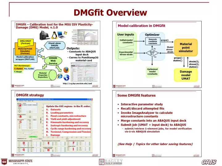
DMGfit – Calibration tool for the MSU ISV Plasticity-Damage (DMG) Model, v.1.0 DMG UMAT (Fortran) Stand-alone DMGfit (MATLAB) Material Point Simulator (Fortran) Outputs: - Constants to ABAQUS input deck - Curves to PamStamp2G material card Model calibration wrapper (MATLAB) DMGfit Web Service M.F. Horstemeyer R.L. Carino Y. Hammi Material Properties Repository T. Haupt http://ccg.hpc.msstate.edu/cmd
Model calibration in DMGfit User inputs Optimizer Initial model constants Generate candidate constants props() Material point simulator Model stress- strain No Experimental stress-strain Good fit ? Yes props() statev() strain(i), stress(i), statev() Optimized model constants Damage model UMAT
DMGfitGUI and calibration strategy Update the GUI regions in the ff. order: • Datasets • Loading parameters • Fixed constants, microstructure • Yield and yield adjustment • Kinematic hardening and recovery • Isotropic hardening and recovery • Cyclic range hardening and recovery • Torsional, Compression and Tension • Damage A B C F E D I G H
Dataset – a text file containing name= value (continuation) # Experimental data (must be the last “name= value”) strain, stress= 0 0 0.00127973 5.73677e+007 0.00248207 1.14556e+008 0.00473197 1.5983e+008 0.00843224 1.88483e+008 0.0129067 2.08455e+008 0.0177175 2.24879e+008 0.0227565 2.39103e+008 0.0280123 2.51231e+008 0.0334448 2.6178e+008 0.039026 2.70922e+008 0.0446936 2.79572e+008 0.0505404 2.86634e+008 0.0565043 2.92804e+008 0.0628393 2.95111e+008 0.0691321 2.98455e+008 0.0755729 3.00528e+008 0.0824714 2.96166e+008 # Format: name= value model_tag= DMG material= az31-ND G= 16666.7 Bulk= 50000 a= 0 b= 0 Tmelt= 3000 heat= 0.34 Kic= 1000 nv= 0.3 fname= MSU1 source= Matt Tucker comment= normal direction excluded= 0 dstype= 1 units= 3 Tinit= 298 dn= 1e-006 fn= 0.001 dcs0= 30 dcs= 30 r0= 0 volF= 0.001 period= 82.4714 rate= 0.001 incr= 100 angle= 0.51 e_load= 0 (continued in next column) More detailed sample datasets in training disc
Typical sequence of steps • Load all experimental datasets. For each dataset, establish the experiment settings (initial temperature, strain rate, stress units, etc), loading parameters, and fixed constants. • First fit the dataset with the lowest temperature and lowest rate. If there are different tests, fit the compression datasets first, followed by tension datasets, then torsion datasets. • For the first dataset, adjust the constants as follows: yield C3; kinematic hardening C9 and recovery C7; isotropic hardening C15 and recovery C13.
Typical sequence of steps (cont) • Restore second dataset. If it has a different temperature than the first, adjust the constants as follows: {C3, C4} if yield is temperature dependent; then {C10, C8, C16, C14}. If the dataset has a different strain rate, adjust C1 and C5 if yield is strain rate dependent, then {C9, C7, C11} and {C15, C13, C17}. • Repeat step 4 for the rest of the datasets. If adjusting the temperature dependence constants (even Cs) does not produce good models for high temperature data, adjust C19 and C20. Adjust torsion, compression and tension differentiation constants, if adding stress state dependent experimental data.
Typical sequence of steps (cont) • Adjust damage constants. To track the evolution of the damage state variable, select Display | Plot a state variable | Damage. Readjust constants in other boxes as necessary. • Record results - Merge constants into an ABAQUS input deck - Write curves to PamStamp2G format - Create comma separated values (CSV), for MS Excel - Create a restart file
DMGfitdemo example - AZ31 Datasets • MSU1: Matt Tucker, 298K, 0.001/s, Tension • MSU2: Matt Tucker, 473K, 0.001/s, Tension • MSU3: Matt Tucker, 298K, 4300/s, Tension • UVA1: Sean Agnew, 373K, 0.05/s, Tension • UVA2: Sean Agnew, 623K, 0.005/s, Tension
Step 1 Load all experimental datasets. For each dataset, establish the experiment settings (initial temperature, strain rate, stress units, etc), loading parameters, and fixed constants.
Load datasets File | Load | A data file … Select datasets
Edit plot settings Stress: 0-600 Legend: NE (northeast)
Step 2 First fit the experimental dataset with the lowest temperature and lowest rate. If there are different tests, fit the compression datasets first, followed by tension datasets, then torsion datasets.
Start with MSU1 (lowest temp, lowest rate dataset) a. Right-click “Exclude” then select “Toggle… datasets” b. Select all, except lowest temp. & lowest rate c. Click OK
The first dataset Click on a data point to display dataset info on left panel Model curve based on default parameters
Step 3 For the first dataset, adjust the constants as follows: • yield C3; • kinematic hardening C9 and recovery C7; • isotropic hardening C15 and recovery C13.
Add kinematic hardening and recovery: C9=10000, C7=1, uncheck; “Apply”; “Optimize”
Add isotropic hardening and recovery: C15=2000, C13=1, uncheck; “Apply”; “Optimize”
Step 4 - Restore second dataset. If it has a different temperature than the first, adjust the constants as follows: • {C3, C4} if yield is temperature dependent; • {C9, C10; C7, C8}; • {C15, C16; C13, C14}. If the dataset has a different strain rate, adjust • C1 and C5 if yield is strain rate dependent; • {C9, C7, C11}; • {C15, C13, C17}.
Add temperature dependence to yield: Estimate C3 & C4 from MSU1 & MSU2 Optimization | Estimate C3 and C4 b. Select MSU1, MSU2 c. Enter 120 for MSU1, 32 for MSU2 d. OK e. OK b a c d e
Add temp. dependence to kinematic hardening & recovery: C10=100, C8=400, uncheck; “Apply”; “Optimize”
Add temp. dependence to isotropic hardening & recovery: C16=100, C14=400, uncheck; “Apply”; “Optimize”
Step 5 Repeat Step 4 for the rest of the datasets. If adjusting the temperature dependence constants (even Cs) does not produce good models for high temperature data, adjust C19 and C20. Adjust torsion, compression and tension differentiation constants, if adding stress state dependent experimental data.
Add rate dependence to yield: C1=5, C2=300, uncheck; “Apply”; “Optimize”
Add rate dependence to kinematic hardening & recovery: C11=0.001, C12=300; check C1, C2; “Apply”; “Optimize”
Example with compression, tension, and torsion data; damage: AL7075-T651
Step 7 Record results. Select File | Write | A “USER MATERIAL, CONSTANTS” for ABAQUS to merge the constants to an existing ABAQUS input deck, or to create a text file containing the constants, suitable for inclusion in an ABAQUS input deck. Select File | Write | A binary restart file to create a record of your session, to resume the session later. Select File | Write | A “fitted constants+ constraints” file to create a text file containing the fitted constants, which may be used as starting values in future fitting sessions. Select File | Write | A post-processing info text file, for import into MS Excel.
Some DMGfit features • Interactive parameter study • Recall/discard attempted fits • Invoke ImageAnalyzer to calculate microstructure constants • Merge constants into an ABAQUS input deck • Submit job (UMAT + input deck) to ABAQUS • submit/retrieve 1-element jobs, for model verification vis-à-vis ABAQUS simulation (See Help | Topics for other labor saving features)
Feature: Interactive “Parameter Study” a. Right-click on value for parameter b. Specify min & max values c. Click on slider to select the current value. d. Enter an exponent for the scale if working with very small or very large values e. Click “Accept” if done, or “Cancel” for no changes b a c e d e
Feature: Navigate attempted fits Navigate the parameter sets Discard current parameter set
Feature: Invoke ImageAnalyzer to calculate microstructure constants The “Fixed constants” may be unique for each dataset. “For all” forces the displayed constants to be used for all datasets.
Feature: Invoke ImageAnalyzer to calculate microstructure constants (cont)
Feature: Merge constants into an existing ABAQUS input deck Example ABAQUS input Manual update of these constants very tedious and error-prone