Download
1 / 26
710 likes | 1.97k Vues
4. Method of Steepest Descent There are two problems associated with the Wiener filtering in practical applications. The matrix inversion operation is difficult to implement. The R and P may not may easy to estimate .

E N D
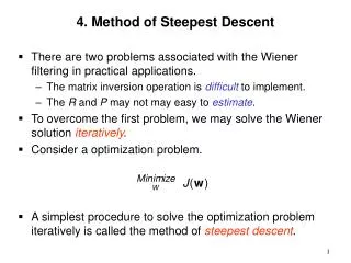
4. Method of Steepest Descent • There are two problems associated with the Wiener filtering in practical applications. • The matrix inversion operation is difficult to implement. • The R and P may not may easy to estimate. • To overcome the first problem, we may solve the Wiener solution iteratively. • Consider a optimization problem. • A simplest procedure to solve the optimization problem iteratively is called the method of steepest descent.
Observation: The gradient of J(w0) corresponds to a direction that has a largest slope at w0.
Method of steepest descent (SD): • Initial guess : w(0) • Compute the gradient vector • update w • Repeat the process (i=i+1) • The parameter is called the step size. It controls the rate of the convergence.
Recall that for the Wiener filtering problem. • Thus, we can use the SD method to solve the Wiener filtering problem. • For real signals, we have
For complex signals, we have • The the update equation for the SD method is • The SD method is a recursive algorithm. It is subject to the possibility of unstable.
Let • The weight update equation can be written as • Since R is the correlation matrix, R=QQH (QHQ=I). • Let v(i)=QHc(i). Then
For the k-th component of v(i), we have • Thus, for vk(i) to converge, it is necessary that • Since all eigenvalues are nonnegative, • To ensure every mode is convergent, we have
Thus, if the step size satisfies the condition, • The time constant (measuring the convergence speed). • Since v(i)=QH[w(i)-wopt], we have
For the i-th component of w(i), we have • Let a be the time constant of wi(i). Then • As we can see that the convergence speed is limited by min. However, we can adjust the step size such that the mode corresponding to max converges fast. • We conclude that the factor control the rate of convergence is the eigenvalue spread (max/min). The smaller the eigenvalue spread, the faster the convergence rate we can achieve.
The MSE can be analyzed similarly. • If the step size is properly chosen, • The curve by plotting J[w(i)] versus i is called the learning curve. The time constant associated with the k-th mode is
Eigenvectors/eigenvalues of R: • Thus, J(w) is a paraboloid. If we cut the paraboloid with planes parallel to w plane [J(w)=constant]. We obtain concentric ellipses. • Let c=w-wopt. Then, vHRv=-Jmin and J=2Rc. Note that J is normal to cHRc. The principle axis of an ellipsoid passes the origin (c=0) and is normal to vTRv. If cp is a principle axis, it must satisfy • Thus, the eigenvectors of R define the principle axes of the error surface.
Geometrical interpretation: c1 v1 c0 v0
The eigenvalues of R give the second derivative of the error surface r.w.t. the principle axes of J=c (what does this mean?). • Thus, if the eigenvalue spread is larger, the shape of the ellipsoid is more peculiar. • Note that • If we can translate and rotate the coordinates of w (to v), components of weights can be decoupled. As a matter of fact, we can use a different step size for different mode. This can have a fastest convergence rate.
Recall the weight update equation. • Let rk=(1-k). Thus, for the k-th mode, the convergence condition is then -1<ck<1.
Weight convergence: underdamped overdamped
Example: identification of AR parameters d(n)=u(n)
Newton’s method • Newton’s method is primarily a method for finding zeros of a equation. • Finding the minimum of a function g(x) means solve the equation g’(x)=0. This leads to the searching algorithm
For the Wiener filtering problem, we have • Thus, Newton’s method is then • As shown, Newton’s method do not proceed in the gradient direction. Introducing the step size, we have Or,
Convergence properties: • Thus, Newton’s method will converge if • Properties • Convergence of Newton’s method is same for every mode and doesn’t dependent on the eigenvalue spread of R. • The computation is more intensive (require R-1). • For nonquadratic cost function, Newton’s method is easy to become unstable.
Question: if we know R-1, we can directly find wopt. Why do we have to use Newton’s method? • Reason: • Exact R-1 may not be necessary. Some efficient methods can be applied to find an approximated of R-1. This is specially true when the input is time-variant. • In general, straightforward Newton’s method is seldom used. Only the concept is adopted.