Download
1 / 39
390 likes | 482 Vues
S-T Connectivity on Digraphs with a Known Stationary Distribution. Kai-Min Chung Harvard University Joint work with: Omer Reingold (Weizmann Inst. of Science) Salil Vadhan (Harvard University). Outline. RL vs. L and s-t connectivity Our main result Derandomization settings

E N D
S-T Connectivity on Digraphs with a Known Stationary Distribution Kai-Min Chung Harvard University Joint work with: Omer Reingold (Weizmann Inst. of Science) Salil Vadhan (Harvard University)
Outline • RL vs. L and s-t connectivity • Our main result • Derandomization settings • Algorithm outline • Main step • Conclusion
Space Space Bounded Complexity Classes L : deterministic logspace Lk : deterministic space O(logk n) RL: randomized logspace polynomial time one-sided error NL: non-deterministic logspace RL vs. L Does randomness help space bounded computation? .. .. .. ... read only .. .. Input: Work: R/W M Random coins 0/1 .. .. .. write only Output: One way
Results on derandomizing space • How much space is sufficient? • RL ⊆ NL ⊆ L2 [Sav70] • RL ⊆L3/2 [Nis92,SZ95] • How many bits can we derandomize? • polylog(n) bits [NZ93] • 2√logn bits with restrictions [RR99] • Make complexity assumptions • RL = L by hardness assumptions[KvM99] • Study s-t connectivity problem
G t s S-T Connectivity (STConn) n: # vertices d: out-degree • Input: (G,s,t) • G – (n,d)-digraph • s,t – vertices in G • Output: does s connect to t?
STConnand logspace computation • Arbitrary digraph • NL-complete • Poly-Mixing digraph • RL-complete [RTV06] • Undirected graph - USTConn • SL-complete [LP82] • USTConn ∈ RL [AKLLR79] • USTConn ∈ L [Rei05]
G t s Random walk algorithm for USTConn [AKLLR79] • Random Walk Algorithm: • Do poly(n) steps random walk from s • Accept if ends at t π(t) is non-negligible converge to stat dist π
Poly-Mixing STConn[RTV06] • Input: (G,s,t,1k) • k: mixing time parameter • YES instance: • s and t are connected • Random walk from s converges to a stationary dist πin k steps • π(s), π(t) ≥ 1/k • NO instance: • No path from s to t Complete for (promise) RL
Graph classes and RL vs. L regular reversible stationary distribution • For what graph class can we solve s-t connectivity in deterministic logspace? • [Rei05] USTConn ∈ L • [RTV06] STConn on regular digraph ∈ L • Our result: Known-Stationary STConn ∈ L
δ-Known-Stationary STConn • Input: (G,s,t,1k,p1,…,pn) • pv: estimate of a stationary dist π(v) (input stationary distribution) • YES instance: • s and t are connected • |pv - π(v)| ≤ δ for all v that can reach s • Random walk from s converges to a stationary dist πs in k steps. • π(s), π(t) ≥ 1/k • No instance: no path from s to t p can be arbitrary
δ-Known-Stationary Find-Path • Input: (G,s,t,1k,p1,…,pn) • YES instance: • s and t are connected • |pv - π(v)| ≤ δ for all v that can reach s • Random walk from s converges to a stationary dist πs in k steps. • π(s), π(t) ≥ 1/k • Output: path from s to t Inspired by [RR99]: estimate of state distribution is available
Our result δ-Known-Stationary STConn and δ-Known-Stationary Find-Path Both in deterministic logspace where δ =1/poly(n,d,k)
Outline • RL vs. L and s-t connectivity • Our main result • Derandomization settings • Algorithm outline • Main step • Conclusion
Explicit vs. oblivious derandomization • Explicit setting • Given input graph explicitly • Oblivious setting • CANNOT look at the graph • Only know parameters of graph • n: #vertices • d: (out-)degree • k: mixing time parameter • Construct PRG for Random Walk Algorithm
Results in explicit settings • Explicit setting • RL ⊆L3/2 [SZ95] • USTConn ∈ L [Rei05] • Known-Stationary STConn ∈ L [Our result]
Results in oblivious settings • Oblivious setting • Nisan’s PRG: O(log2 n) seed length [Nis92] • RTV’s PRG: O(log n) seed length, only for regular digraph w/ “consistent labelling” (based on Reingold’s approach) [RTV06] • PRG for regular digraph w/ arbitrary labelling ⇒ RL = L [RTV06] • Other applications [Ind00,KNO05,…]
Outline • RL vs. L and s-t connectivity • Our main result • Derandomization settings • Algorithm outline • Main step • Conclusion
δ-Known-Stationary Find-Path • Input: (G,s,t,1k,p1,…,pn) • YES instance: • s and t are connected • |pv - π(v)| ≤ δ for all v that can reach s • Random walk from s converges to a stationary dist πs in k steps. • π(s), π(t) ≥ 1/k • Output: path from s to t
Overview • Main idea: • Use stationary distribution to convert G to nearlyregular, “consistently labelled” graph so that we can apply RTV’s PRG • Challenges: • Logspace construction • Maintain mixing time
Algorithm Logspace G G’ G’’ ε ε nearly regular Gcon Greg Analysis Step 1: use input stationary distribution to convert G to nearly regularG’
Algorithm Apply PRG Logspace G G’ G’’ ε ε a path from s to t Gcon Greg Analysis Step 2: apply PRG to G’, and project path to G
Actually… Apply PRG Logspace G G’ G’’ ε ε consistently labelled Gcon Greg Analysis Need to obtain “consistent labelling” But this is easy!
Analysis: PRG can find a path on G’ Logspace Error: ε⋅#step G G’ G’’ Apply PRG PRG works! ε ε Gcon Greg Analysis G’ ≈ Greg PRG works for Greg ⇒ PRG works for G’
Maintain mixing time Logspace G G’ G’’ Maintain mixing-time Maintain mixing-time ε ε Gcon Greg Analysis Mixing time: G ≈ G’ ≈ Greg New mixing time measure: visiting length.
Outline • RL vs. L and s-t connectivity • Our main result • Derandomization settings • Algorithm outline • Main step • Conclusion
Stationary dist as network flow • Vertex v has mass π(v) • Edge (v,w) carries π(v)/d flow • Regular ⇔ uniform dist is stationary ⇔ vertices have equal mass & edges carry equal flow 0.2 0.1 0.1 0.2 0.2 0.1 0.1 0.2 0.2 0.1
Ideal construction • Blow up each v to cloud Cvof size π(v)⋅N • Each v’ ∈Cv has equal mass 1/N G 4/7 1/7 1/7 2/7 1/7 1/7 1/7 1/7 1/7 1/7
Ideal construction • Blow up each v to cloud Cv of size π(v)⋅N • Each v’ ∈Cv has equal mass 1/N • Each vertex has a copy of outgoing edges 1/7 1/7 1/7 1/7 1/7 1/7 1/7 1/7
Ideal construction • Blow up each v to cloud Cv of size π(v)⋅N • Each v’ ∈Cv has equal mass 1/N • Each vertex has a copy of outgoing edges • Split each outgoing edge into D edges, distributed evenly to target cloud • Each edge shares equal 1/(dDN) flow Regular! G’ 1/7 1/7 1/7 1/7 1/7 1/7 1/7 1/7
Ideal construction rounding error rounding error • Blow up each v to cloud Cv of size π(v)⋅N • Each v’ ∈Cv has equal mass 1/N • Each vertex has a copy of outgoing edges • Split each outgoing edge into D edges, distributed evenly to the target cloud • Each edge shares equal 1/(dDN) flow negligible probability G’ 1/7 1/7 1/7 1/7 1/7 1/7 1/7 1/7
G’ is nearly regular • There are ε-fraction of bad vertices with small degree • For every good vertex • (1- ε)dD ≤ outdeg ≤ dD • (1- ε)dD ≤ indeg ≤ (1+ ε)dD
G’ maintains mixing time • Visiting length k • A mixing time measure • The construction maintains the visiting length • visiting len. of G’ = visiting len. of G
G S v Visiting length • k(S) : visiting length of a vertex set S • For every v reachable from S Pr[ v visits S in k(S) steps ] ≥ ½ Lemma: mix in time poly(k)⋅log(nd) if S is a clique.
G ⇒ G’ maintains visiting length • visiting length k(Cs) in G’ = visiting length k(s) in G • On the cloud level, G’ = G • Pr[ Cv to Cw in G’] = Pr[ v to w in G] ⇒G’ has short mixing time • independent of ε G’ vs. G
Recap Apply PRG Logspace G G’ G’’ ε ε Gcon Greg Analysis Apply PRG to G’ to find a path
Outline • RL vs. L and s-t connectivity • Our main result • Derandomization settings • Algorithm outline • Conclusion
Conclusion • Key to Reingold’s approach • Oblivious: consistent labelling of edges • Explicit: knowledge of stationary dist • Toward RL = L • Focus on unknown stationary dist • Put RL in L1.4?
Thank you! Questions?