Download
1 / 12
130 likes | 268 Vues
Chapter 13 – Behavior of Spectral Lines. We began with line absorption coefficients which give the shapes of spectral lines. Now we move into the calculation of line strength from a stellar atmosphere. Formalism of radiative transfer in spectral lines Transfer equation for lines

E N D
Chapter 13 – Behavior of Spectral Lines We began with line absorption coefficients which give the shapes of spectral lines. Now we move into the calculation of line strength from a stellar atmosphere. • Formalism of radiative transfer in spectral lines • Transfer equation for lines • The line source function • Computing the line profile in LTE • Depth of formation • Temperature and pressure dependence of line strength • The curve of growth
The Line Transfer Equation • We can add the continuous absorption coefficient and the line absorption coefficient to get the total absorption coefficient: dtn = (ln+kn)rdx • And the source function as the sum of the line and continuous emission coefficients divided by the sum of the line and continuous emission coefficients. • Or define the line and continuum source functions separately: • Sl=jnl/ln • Sc=jnc/kn • In either case, we still have the basic transfer equation:
The Line Source Function • The basic problem is still how to obtain the source function to solve the transfer equation. • But the line source function depends on the atomic level populations, which themselves depend on the continuum intensity and the continuum source function. This coupling complicates the solution of the transfer equation for lines. • Recall that in the case of LTE the continuum source function is just the Bn(T), the Planck Function. • The assumption of LTE simplifies the line case in the same way, and allows us to describe the energy level populations strictly by the temperature without coupling to the radiation field. • This approximation works when the excitation states of the gas are defined primarily by collisions and not radiative excitation or de-excitation.
Mapping the Line Source Function • The line source function with depth maps into the line profile • The center of the line is formed at shallower optical depth, and maps to the source function at smaller t • The wings of the line are formed in progressively deeper layers
Computing the Line Profile • The line profile results from the solution of the transfer equation at each Dl through the line. • The line profile will depend on the number of absorbers at each depth in the atmosphere • The simplifying assumptions are • LTE • Pure absorption (no scattering) • How well does this work? • To know for sure we must compute the line profile in the general case and compare it to what we get with simplifying assumptions • Generally, it’s pretty good • Start with the assumed T(t) relation and model atmosphere • Recompute the flux using the line+continuous opacity at each wavelength around the line • For blended lines, just add the line absorption coefficients appropriate at each wavelength
Depth of Formation • It’s straightforward to determine approximately where in the atmosphere (in terms of the optical depth of the continuum) each part of the line profile is formed • But even at a specific Dl, a range of optical depths contributes to the absorption at that wavelength • It’s not straightforward to characterize the depth of formation of an entire line • The cores of strong lines are formed at very shallow optical depths.
The Ca II K Line @ 3933A • Why does the line have an emission peak (a reversal) in the center? • In the Sun, the central emission peak is self-absorbed. Why?
The Behavior of Line Strength • The strengths of spectral lines depend on • The width of the absorption coefficient • Thermal and microturbulent velocities • The number of absorbers • Temperature • Electron pressure or luminosity • Atomic constants • In strong lines – collisional line broadening affected by the gas and electron pressures
The Effect of Temperature • Temperature is the main factor affecting line strength • Exponential and power of T in excitation and ionization • Increase with T due to increase in excitation • Decrease beyond maximum an increase in the opacity or from ionization
H-g Profiles • H lines are sensitive to temperature because of the Stark effect The high excitation of the Balmer series (10.2 eV) means excitation continues to increase to high temperature (max at ~ 9000K). Most metal lines have disappeared by this temperature. Why?
How do different kinds of lines behave with temperature? • Lines from a neutral species of a mostly neutral element • Lines from a neutral species of a mostly ionized element • Lines from an ion of a mostly neutral element • Lines from an ion of a mostly ionized element • Consider gas with H- as the dominant opacity
Neutral lines from a neutral species • Number of absorbers proportional to exp(-c/kT) • Number of neutrals independent of temperature (why?) • Ratio of line to continuous absorption coefficient • But Pe is ~ proportional to exp(T/1000), so…