Download
1 / 78
800 likes | 808 Vues
CSCE 441: Computer Graphics Forward/Inverse kinematics. Jinxiang Chai. Outline. Animation basics: Forward kinematics Inverse kinematics. Kinematics. The study of movement without the consideration of the masses or forces that bring about the motion. Animation.

E N D
CSCE 441: Computer Graphics Forward/Inverse kinematics Jinxiang Chai
Outline Animation basics: • Forward kinematics • Inverse kinematics
Kinematics The study of movement without the consideration of the masses or forces that bring about the motion
Animation • Robot arm animation (click here) • Pixar lamp animation (click here)
Degrees of Freedom (Dofs) The set of independent displacements that specify an object’s pose
Degrees of Freedom (Dofs) The set of independent displacements that specify an object’s pose • How many degrees of freedom when flying?
Degrees of Freedom (Dofs) The set of independent displacements that specify an object’s pose • How many degrees of freedom when flying? • So the kinematics of this airplane permit movement anywhere in three dimensions • Six • x, y, and z positions • roll, pitch, and yaw
Degrees of Freedom • How about this robot arm? Click (here) • Six • 2-shoulder, 1-elbow, 3-wrist
Configuration Space vs. Work Space • Configuration space • The space that defines the possible object configurations • Degrees of Freedom • The number of parameters that are necessary and sufficient to define position in configuration • Work space • The space in which the object exists • Dimensionality • R3 for most things, R2 for planar arms
Forward vs. Inverse Kinematics • Forward Kinematics • Compute configuration (pose) given individual DOF values • Inverse Kinematics • Compute individual DOF values that result in specified end effector’s position
End Effector Base Example: Two-link Structure • Two links connected by rotational joints θ2 l2 l1 θ1 X=(x,y)
End Effector Base Example: Two-link Structure • Animator specifies the joint angles: θ1θ2 • Computer finds the position of end-effector: x θ2 l2 l1 θ1 X=(x,y) (0,0) x=f(θ1, θ2)
End Effector Base Example: Two-link Structure • Animator specifies the joint angles: θ1θ2 • Computer finds the position of end-effector: x θ2 θ2 l2 l1 θ1 X=(x,y) (0,0) x = (l1cosθ1+l2cos(θ2+ θ2) y = l1sinθ1+l2sin(θ2+ θ2))
End Effector Base Forward Kinematics • Create an animation by specifying the joint angle trajectories θ2 θ2 l2 l1 θ1 X=(x,y) (0,0) θ1 θ2
Forward Kinematics lower arm middle arm Upper arm base A 2D lamp with 6 degrees of freedom
Base Inverse Kinematics • What if an animator specifies position of end-effector? θ2 θ2 l2 l1 End Effector θ1 X=(x,y) (0,0)
Base Inverse Kinematics • Animator specifies the position of end-effector: x • Computer finds joint angles: θ1θ2 θ2 θ2 l2 l1 End Effector θ1 X=(x,y) (0,0) (θ1, θ2)=f-1(x)
Base Inverse Kinematics • Animator specifies the position of end-effector: x • Computer finds joint angles: θ1θ2 θ2 θ2 l2 l1 End Effector θ1 X=(x,y) (0,0)
Why Inverse Kinematics? • Motion capture • Basic tools in character animation - key frame generation - animation control - interactive manipulation • Computer vision (video-based mocap) • Robotics • Bioinfomatics (Protein Inverse Kinematics) • Etc.
Inverse Kinematics • Given end effector’s positions, compute required joint angles • In simple case, analytic solution exists • Use trig, geometry, and algebra to solve
Inverse Kinematics • Analytical solution only works for a fairly simple structure • Numerical/iterative solution needed for a complex structure
Numerical Approaches • Inverse kinematics can be formulated as an optimization problem
Function Optimization • Finding the minimum for nonlinear functions F(x) x
Optimization As a Tool • How to use optimization to solve the following linear system? 3x + 2y = 5; 4x – 5y = 6
Optimization As a Tool • How to use optimization to solve the following linear system? 3x + 2y = 5; 4x – 5y = 6 Define a function: F(x,y) = (3x+2y-5)2+(4x-5y-6)2
Optimization As a Tool • How to use optimization to solve the following linear system? 3x + 2y = 5; 4x – 5y = 6 Could be nonlinear equations! Define a function: F(x,y) = (3x+2y-5)2+(4x-5y-6)2 Finding the minimum for F(x,y) : x+,y+= argminx,y (3x+2y-5)2+(4x-5y-6)2
Optimization As a Tool • How to use optimization to solve the following linear system? f(x, y) = 0; g(x,y) = 0 Could be nonlinear equations! Define a function: F(x,y) = f(x,y)2+g(x,y)2 Finding the minimum for F(x,y) : x+,y+= argminx,y f(x,y)2+g(x,y)2
Base Formulation • So how to convert the IK process into an optimization function? Find the pose satisfying: θ2 θ2 l2 l1 θ1 C=(Cx,Cy) (0,0)
Base Iterative Approaches Find the joint angles θ that minimizes the distance between the hypothesized character position and user specified position hypothesized position specified position θ2 θ2 l2 l1 θ1 C=(Cx,Cy) (0,0)
Base Iterative Approaches Find the joint angles θ that minimizes the distance between the hypothesized character position and user specified position θ2 θ2 l2 l1 θ1 C=(c1,c2) (0,0)
Iterative Approaches Mathematically, we can formulate this as an optimization problem: The above problem can be solved by many nonlinear optimization algorithms: - Steepest descent - Gauss-newton - Levenberg-marquardt, etc
Gauss-Newton Approach Step 1: initialize the joint angles with Step 2: update the joint angles until the solution converges:
Gauss-Newton Approach Step 1: initialize the joint angles with Step 2: update the joint angles until the solution converges: How can we decide the amount of update?
Gauss-Newton Approach Step 1: initialize the joint angles with Step 2: update the joint angles:
Gauss-Newton Approach Step 1: initialize the joint angles with Step 2: update the joint angles: Known!
Gauss-Newton Approach Step 1: initialize the joint angles with Step 2: update the joint angles: Taylor series expansion
Gauss-Newton Approach Step 1: initialize the joint angles with Step 2: update the joint angles: Taylor series expansion rearrange
Gauss-Newton Approach Step 1: initialize the joint angles with Step 2: update the joint angles: Taylor series expansion: linear approximation rearrange Can you solve this optimization problem?
Gauss-Newton Approach Step 1: initialize the joint angles with Step 2: update the joint angles: Taylor series expansion rearrange This is a quadratic function of
Gauss-Newton Approach • Optimizing an quadratic function is easy • It has an optimal value when the gradient is zero
Gauss-Newton Approach • Optimizing an quadratic function is easy • It has an optimal value when the gradient is zero b J Δθ Linear equation!
Gauss-Newton Approach • Optimizing an quadratic function is easy • It has an optimal value when the gradient is zero b J Δθ
Gauss-Newton Approach • Optimizing an quadratic function is easy • It has an optimal value when the gradient is zero b J Δθ
Jacobian Matrix • Jacobian maps the velocity in joint angle space to velocities in Cartesian space (x,y) A small change of θ1and θ2results in how much change of end-effector position (x,y) θ2 θ1
Jacobian Matrix • Jacobian maps the velocity in joint angle space to velocities in Cartesian space (x,y) A small change of θ2results in how much change of end-effector position f=(x,y) θ2 θ1
Base Jacobian Matrix: 2D-link Structure θ2 θ2 l2 l1 θ1 C=(c1,c2) (0,0)
Base Jacobian Matrix: 2D-link Structure θ2 θ2 l2 l1 θ1 C=(c1,c2) (0,0) f2 f1
Base Jacobian Matrix: 2D-link Structure θ2 θ2 l2 l1 θ1 C=(c1,c2) (0,0)
Base Jacobian Matrix: 2D-link Structure θ2 θ2 l2 l1 θ1 C=(c1,c2) (0,0)