Download
1 / 35
360 likes | 597 Vues
Lecture 14 Models II. Principles of Landscape Ecology March 31, 2005. Raster models. Individual tree models. Spatially dynamic. X LANDIS-II. Patch models. Gap models. Mechanistic detail. Cellular Models. A system of cell networks or grids Cells interact with neighborhood

E N D
Lecture 14Models II Principles of Landscape Ecology March 31, 2005
Raster models Individual tree models Spatially dynamic X LANDIS-II Patch models Gap models Mechanistic detail
Cellular Models • A system of cell networks or grids • Cells interact with neighborhood • Each cell adopts one of m (m may be infinite) possible states • Transition rules for each state can be simple, deterministic, or stochastic. • Transition rules ~ f(abiotic constraints, biotic interactions, disturbances)
What is a cellular landscape model? Cellular landscape models simulate change through time in response to endogenous processes (growth, competition) and exogenous forcing (disturbance, climate change, etc). • Spatially explicit and spatially interactive • GIS used to store/display data. • Entities have map coordinates • Include spatial processes: seed dispersal, disturbance • Run iteratively over time • The landscape has a memory of previous events • ‘Equilibrium’ doesn’t apply in the sense of analytical models
30 m Model Example: LANDIS-II • Spatially interactive cellular model • Each site exchanges information (seeds) and energy (disturbances: chemical and mechanical) with neighboring sites. • Species have unique life history attributes • -shade tolerance, fire tolerance • -longevity, maturity age • -seed dispersal capabilities • Species presence in age cohorts. • Example: sugar maple 11-20, 41-50 + • basswood 61-70, 101-110
FORESTED LANDSCAPE DISPERSAL SPECIES ESTABLISHMENT INSECTS / DISEASE CLIMATE LIVING BIOMASS HARVESTING FIRE DEAD BIOMASS WINDTHROW Model Example: LANDIS-II • Multiple disturbances and interactions • Scales tree growth up to the landscape scale
Model Application Example: Climate change effects in northern Wisconsin • Goal: • Estimate the effects of climate change and disturbance on forest composition and biomass.
Potential Great Lakes Forests Spp composition Aboveground - Biomass Current Great Lakes Forests CLIMATE CHANGE Forest tree communities Disturbance Dispersal Ecosystem Processes Scenarios • Why Species Composition and Biomass? • Of concern to management • Integrating variables
Simulation of climate change in northern Wisconsin • Climate change effects modeled: • tree species germination and establishment • tree spp growth rates and competitive ability • Climate change effects not modeled: • changes in disturbance regimes • potential CO2 fertilization • changes in soil properties Other processes not modeled: • herbivory • exotic species
Climate Scenarios • 3 climate scenarios: • Current Climate • Hadley Centre for Climate Prediction +3.8°C and +38cm ppt • Canadian Centre for Climate Modelling +5.8°C and +20cm ppt Simulate forest change over 200 years • Years 1990 - 2090 includes climate change • Constant climate from 2090 - 2190 • 10 year climate averages
Disturbance Scenarios • Two Disturbance Scenarios: • No Disturbance • Wind + Harvesting • Wind equal to historic frequency • Clearcutting • Selective cutting • Heavy thinning
LANDIS-II Input Data 23 tree species with life history attributes Probability of establishment calculated from a forest gap model (0.1 ha) Growth and decomposition rates Establishment, growth, and decomposition varied among ecoregions due to climate and soils
270 45 90 225 180 > 325 Mg/ha 135 Total Aboveground Live Biomass Canadian GCM No Disturbance Wind and Harvesting ANIMATION Aboveground Live Biomass
270 45 90 225 180 > 325 Mg/ha 135 Total Aboveground Live Biomass Canadian GCM No Disturbance Wind and Harvesting Aboveground Live Biomass
Current Climate Hadley Climate Canadian Climate Results: Biomass change constant climate begins Without Disturbance With Wind & Harvesting
Results: Change in community composition • Without Disturbance: • The landscape becomes dominated by sugar maple • Few opportunities for southern species to migrate north • With Wind and Harvesting: • Shift toward southern oak and hickory if climate changes, although the shift is small
At the same time, many species will be displaced. As climate changes, we expect northward migration of some tree species. Interactions between climate change and fragmentation Wisconsin Illinois
Interactions between climate change and fragmentation However, species migration limited by: • distance-limited seed dispersal • the priority effect - occupancy by current species Other limits not considered: • generational lags • herbivory Wisconsin Illinois
Interactions between climate change and fragmentation Wisconsin • Fragmentation also reduces migration: • fewer available colonization sites • fewer seed sources Illinois
Interactions between climate change and fragmentation Consequences: Spp richness reduced. Decline in productivity and aboveground live biomass. Why? Realized niche <> fundamental niche. The species best adapted to new climate are not widely dispersed. Wisconsin Illinois
Interactions between climate change and fragmentation Our Questions: How will seed dispersal limitations affect aboveground live biomass? Is seed dispersal limited by fragmentation? Is seed dispersal limited by existing species? Wisconsin Illinois
Estimation of the effects of seed dispersal How do we measure the effect that seed dispersal has on aboveground live biomass (B)? Estimate B from identical scenarios with distance limited seed dispersal and without seed dispersal distance limitations. Calculate Difference Total Bno distance limit - Total Bdistance limited = Total Bseed dispersal effect
Hadley Climate Canadian Climate Estimation of the effects of seed dispersal
Climate Change Conclusions • Disturbance is a strong determinant of future community composition under climate change. • But, five important tree species will be extirpated and landscape diversity will be reduced if the climate warms.
Climate Change Conclusions • The northward migration of many species is limited by seed dispersal. • Aboveground live biomass is limited by seed dispersal. • Management will need to balance carbon storage, maintenance of diversity, and the reality of species loss.
Caveats: • Only two possible climate change scenarios out of dozens. • We did not include many critical processes, e.g. herbivores. • Our results are unvalidated. Question: What, if any, value does this research have for management?
Modeling Conclusions Preparing input data is the most arduous task. Garbage in, garbage out (?). Replication is not always helpful - depends on the size of stochastic events. You can never include everything. Always focus on the questions first, tools last.
Modeling Conclusions • Technical limitations remain • Increase in computer capability in past decade is not a panacea. • Challenge of appropriate complexity in spatial models remains • Spatial data availability • Spatial and temporal scale limitations • Resolution—Extent tradeoff
Model caveats http://www.env.duke.edu/landscape/classes/env214/le_mod0.html
Building model confidence: data validation • Traditional validation: compare model data with empirical data. However, there is rarely independent landscape data collected at same scales. Data solutions include: • Fine-scale data • Problem:wrong scale • Space-for-time • e.g. southern forests ~ climate change • Problem:different initial conditions, multiple changes • Reconstruct past responses • Problem:unknown starting conditions • lack of human behavior model • lack of climate data • Compare to other models • e.g. GCMs • Problem:few other FLSMs applied at regional scale • Both models wrong or right? Model autocorrelation.
Building model confidence: alternatives to validation • Landscape validation is not always possible - need to judge by different standards. • Process validation • Independent application, assessment, and review • Indirect Corroborating evidence • Development over time • Model transparency: • open code • generous comments
Building model confidence: Summary Model acceptance • Confidence from: • application • review • development • mistakes! + Doubts from increasing complexity - Model development time