Download

1 / 20
290 likes | 679 Vues
Normal Distribution . Chapter 3. Density Curves. Example: here is a histogram of vocabulary scores of 947 seventh graders. The smooth curve drawn over the histogram is a mathematical model for the distribution. Density Curves.

E N D
Normal Distribution Chapter 3
Density Curves Example: here is a histogram of vocabulary scores of 947 seventh graders. The smooth curve drawn over the histogram is a mathematical modelfor the distribution. Chapter 3
Density Curves Example: the areas of the shaded bars in this histogram represent the proportion of scores in the observed data that are less than or equal to 6.0. This proportion is equal to 0.303. Chapter 3
Density Curves Example: now the area under the smooth curve to the left of 6.0 is shaded. If the scale is adjusted so the total area under the curve is exactly 1, then this curve is called a density curve. The proportion of the area to the left of 6.0 is now equal to 0.293. Chapter 3
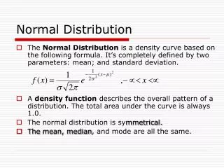
DENSITY CURVE A density curve is a curve that • is always on or above the horizontal axis, and • has area exactly 1 underneath it. A density curve describes the overall pattern of a distribution. The area under the curve and above any range of values is the proportion of all observations that fall in that range. A normal distribution is described by a density curve that is a continuous, symmetric, bell-shaped distribution of a variable.
A normal distribution curveis the theoretical counterpart to a relative frequency histogram for a large number of data values with a very small class width.
Properties of a Normal Distribution A normal distribution curve is bell-shaped The mean, median, and mode are equal and are located at the center of the distribution A normal distribution curve is unimodal (i.e., it has only one mode) The curve is symmetric about the mean, which is equivalent to saying that its shape is the same on both sides of a vertical line passing through the center The curve is continuous, that is, there are no gaps or holes. For each value of X, there is a corresponding value of Y The curve never touches the x axis. Theoretically, no matter how far in either direction the curve extends, it never meets the x axis – but it gets increasingly closer The total area under a normal distribution curve is equal to 1.00, or 100% The Empirical Rule applies
The Empirical Rule68-95-99.7 Rule The area under the part of a normal curve that lies within 1 standard deviation of the mean is approximately 0.68, or 68%; within 2 standard deviations, about 0.95, or 95%; and within 3 standard deviations, about 0.997, or 99.7%.
What shapes the curve? The standard deviation σ, is the natural measure of spread for the Normal Distribution. Between µ – σ, and µ + σ, (in the center of the curve), the graph curves downward. The graph curves upward to the left of µ – σ, and to the right of µ + σ. The points at which the curve changes from curving upward to curving downward are called the inflection points.
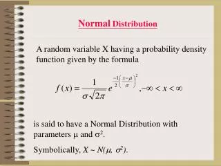
Standardizing the Normal Distribution A z-score tells us how many standard deviations the original observation falls away from the mean, and in which direction. Observations larger than the mean are positive when standardized, and observations smaller than the mean are negative. If x is an observation from a distribution that has mean μ and standard deviation σ, that is N(μ, σ), the standardized valueof x is A standardized value is often called a z-score. The standard normal distribution of the new value is the normal distribution N(0,1) with mean 0 and standard deviation 1.
Area Under the Normal Curve The proportion of observations on a standard normal variable, z can be taken from the area under the normal curve. The cumulative proportion for a value x in adistribution is the proportion of observations in the distribution that are less than or equal to x. The area for the cumulative proportion is usually found from a table of areas. The entry for each value x is the area under the curve to the left of x.
Example 1 – Find the Area Table A – Cumulative Probability What proportion of observations on a standard Normal variable z take values less than 1.47? Solution: To find the area to the left of 1.47, locate 1.4 in the left-hand column of Table A, then locate the remaining digit 7 as .07 in the top row. The entry opposite 1.4 and under .07 is 0.9292.
Example 2 – Who qualifies for college sports? Scores of high school seniors on the SAT follow the Normal distribution with mean μ = 1026 and standard deviation σ = 209. These seniors qualify for NCAA sports with a score of 820. What percent of seniors scored at least 820? Step 1. Draw a picture. Step 2. Standardize. Call the SAT score x. Subtract the mean, then divide by the standard deviation, to transform the problem about x into a problem about a standard Normal z: Step 3. Use the table. The picture shows that we need the cumulative proportion for x = 820. Step 2 says this is the same as the cumulative proportion for z = − 0.99. The Table A entry for z = − 0.99 says that this cumulative proportion is 0.1611. The area to the right of − 0.99 is therefore 1 − 0.1611 = 0.8389. So 84% of high school seniors scored at least 820.
Example 3 – Who qualifies for college sports? The NCAA considers a student a “partial qualifier” for Division II athletics if high school grades are satisfactory and the combined SAT score is at least 720. What proportion of all students who take the SAT would be partial qualifiers? Step 1. Draw a picture. Call the SAT score x. The variable x has the N(1026, 209) distribution. What proportion of SAT scores fall between 720 and 820? Here is the picture: Step 2. Standardize. Subtract the mean, then divide by the standard deviation, to turn x into a standard Normal z: Step 3. Use the table. area between −1.46 and −0.99 = (area left of −0.99) − (area left of −1.46) = 0.1611 − 0.0721 = 0.0890 About 9% of high school seniors would be partial qualifiers.
.10 ? 70 (height values) Example 4 - Health and Nutrition Examination Study of 1976-1980 How tall must a man be to place in the lower 10% for men aged 18 to 24? Chapter 3
Table A:Standard Normal Probabilities Look up the closest probability (to .10 here) in the table. Find the corresponding standardized score. The value you seek is that many standard deviations from the mean. .08 1.2 .1003 Chapter 3
.10 ? 70 (height values) Example 4 - Health and Nutrition Examination Study of 1976-1980 • How tall must a man be to place in the lower 10% for men aged 18 to 24? -1.28 = z (standardized values) Chapter 3
Observed Value for a Standardized Score • Need to “unstandardize” the z-score to find the observed value (x) : • observed value = mean plus [(standardized score) (stddev)] Chapter 3
Observed Value for a Standardized Score • observed value = mean plus [(standardized score) (std dev)] = 70 + [(-1.28 ) (2.8)] = 70 + (3.58) = 66.42 • A man would have to be approximately 66.42 inches tall or less to place in the lower 10% of all men in the population. Chapter 3