Download
1 / 32
320 likes | 454 Vues
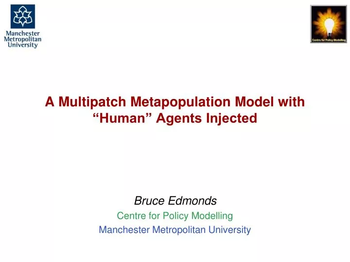
A Multipatch Metapopulation Model with “Human” Agents Injected. Bruce Edmonds Centre for Policy Modelling Manchester Metropolitan University. Motivation. Complex Individual-based Model. Complex Individual-based Model. Socio-Ecological Model. Combined Complex Model. Social Model.

E N D
A MultipatchMetapopulation Model with “Human” Agents Injected Bruce Edmonds Centre for Policy Modelling Manchester Metropolitan University
Motivation Complex Individual-based Model Complex Individual-based Model Socio-Ecological Model Combined Complex Model Social Model SimpleSystem-dynamics Model SimpleSystem-dynamics Model Ecological Model
Model of Ecology Slow random rate of migration between patches Each individual represented separately A well-mixed patch • A wrapped 2D grid of well-mixed patches with: • energy (transient) • bit string of characteristics • Organisms represented individually with its own characteristics, including: • bit string of characteristics • energy • position • stats recorders
Model sequence each simulation tick • Input energy equally divided between patches. • Death. A life tax is subtracted, some die, age incremented • Initial seeding. until a viable is established, random new individual • Energy extraction from patch. energy divided among the individuals there with positive score when its bit-string is evaluated against patch • Predation. each individual is randomly paired with a number of others on the patch, if dominate them, get a % of their energy, other removed • Maximum Store. energy above a maximum level is discarded. • Birth. Those with energy > “reproduce-level” gives birth to a new entity with the same bit-string as itself, with a probability of mutation, Child has an energy of 1, taken from the parent. • Migration. randomly individuals move to one of 4 neighbours • Statistics. Various statistics are calculated.
Key advantages of this • Produces a complex space of changing food webs • Model creates endogenous shocks and unpredictable adaptions (to, for example, man) • Species arms-races, predator-prey dynamics, waves of species spread etc. all exhibited • Levels of environmental variety, size, granularity etc. are determined by paramters • Mutation and migration happen in parallel • “Equilibrium” almost never observed • Diversity of ecologies are emergent outcomes • “Human” agents can be embedded in food chains and the combined complexity of this explored
Non-Viable Ecology Typical Non-Viable Ecologythe world state (left) Number of Species (centre) Log, 1 + Number of Individuals at each trophic level (right)
Dominant Species Ecology TypicalDominant Species Ecology the world state (left) Number of Species (centre) Log, 1 + Number of Individuals at each trophic level (right)
Rich Plant Ecology Typical Rich Plant Ecologythe world state (left) Number of Species (centre) Log, 1 + Number of Individuals at each trophic level (right)
Mixed Ecology Typical Mixed Ecology the world state (left) Number of Species (centre) Log, 1 + Number of Individuals at each trophic level (right)
Neutral patches, random migration, plants only • As predicted by Hubble’s “Neutral Theory” • “skewed s-shaped” relative species abundance curve • “Multinomial distribution” of log2 species distribution • Except, maybe, species-area scatter chart
Neutral Patches, local migration, plants only • unchanged “skewed s-shaped” relative species abundance curve • “Multinomial distribution” of log2 species distribution but with more lower abundance species • Pretty flat species-area scatter plot
Selective patches, random migration, plants only • “Linear” drop in log 2 species abundance • “Exponential” shaped relative species abundance graph • Flatter species area scatter plot
Neutral Patches, random migration, predators • Lots of new species plus flatter log 2 species distribution • flat or curved species abundance distribution • a variety of species-area curves
Adding “Human” Agents • The agents representing humans are “injected” (as a group) into the simulation once an ecology of other species has had time to evolve • The state of the ecology is then evaluated some time later or over a period of time • These agents are the same as other individual in most respects, including predation but “humans”: • can change their bit-string of skills by imitating others on the same patch (who are doing better than them) • might have a higher “innovation” rate than mutation • might share excess food with others around • might have different migration rates etc. • Could have many other learning, reasoning abilities
Example run with: selective environment, local migration, predators, and “humans” @ tick 2000 @tick2000 – before “humans” @tick5000 – after “humans”
Effect of humans vs. environmental complexity proportion of ecology types, red=plant, blue=mixed, purple=single species, green=non-viable diversity of ecology, blue=with humans, red=without
Effect of humans vs. general migration rate proportion of ecology types, red=plant, blue=mixed, purple=single species, green=non-viable diversity of ecology, blue=with humans, red=without
Effect of humans vs. food input to world proportion of ecology types, red=plant, blue=mixed, purple=single species, green=non-viable diversity of ecology, blue=with humans, red=without
Human migr. rate vs. diversity (all with humans, other entities having 0.1 migration rate)
Starting from plant ecology (with humans) Starting from a Plant Ecology the effects of innovation rate/mutation rate (left) and people migration rate/entity migration rate (right) , red=plant, blue=mixed, purple=single species, green=non-viable
Starting from mixed ecology (with humans) Starting from a Mixed Ecology the effects of innovation rate/mutation rate (left) and people migration rate/entity migration rate (right) , red=plant, blue=mixed, purple=single species, green=non-viable
Starting from single species ecology (with humans) Starting from a Single Species Ecology the effects of innovation rate/mutation rate (left) and people migration rate/entity migration rate (right) , red=plant, blue=mixed, purple=single species, green=non-viable
The End! Bruce Edmonds:http://bruce.edmonds.name Centre for Policy Modelling:http://cfpm.org A paper describing some of this, the model, these slides at:http://cfpm.org/cpmrep222.html